Python Reference

Useful Python Commands for Differential Equations

Note

This page is a quick-reference guide to Python tools used throughout this course. It is not a complete Python tutorial. Students who want a deeper introduction may find the following resources helpful:

Installing and Managing Python and Packages

Python (Python Software Foundation 2024) can be installed and managed in several ways. Below we describe two popular approaches: uv (a modern, fast tool) and conda (a traditional choice popular in scientific computing). Either approach works fine for this course.

Option 1: `uv` (Recommended for New Users)

uv is a fast, modern Python package and project manager written in Rust. It can install Python itself, create isolated project environments, and manage packages — all in one tool.

Installing uv:

On macOS and Linux (run in your terminal):

curl -LsSf https://astral.sh/uv/install.sh | sh

On Windows (run in PowerShell):

powershell -ExecutionPolicy ByPass -c "irm https://astral.sh/uv/install.ps1 | iex"

Installing Python with uv:

uv python install 3.14   # installs Python 3.14

Creating a virtual environment and installing packages:

A virtual environment is an isolated folder that holds a specific Python version and a set of packages for a project. This keeps your projects from interfering with each other.

# Create a new project folder and enter it
mkdir my_diffeq_project
cd my_diffeq_project

# Create a virtual environment using a specific Python version
uv venv --python 3.14

# Activate the environment
# On macOS/Linux:
source .venv/bin/activate
# On Windows:
.venv\Scripts\activate

# Install packages needed for this course
uv pip install numpy scipy sympy matplotlib

# Deactivate when you're done working
deactivate

Registering the environment as a Jupyter kernel (so it appears in VS Code or JupyterLab):

uv pip install ipykernel
python -m ipykernel install --user --name diffeq_py --display-name "DiffEq Python"

For full documentation see https://docs.astral.sh/uv/.

Option 2: `conda` / Anaconda

Conda is a package and environment manager that is widely used in scientific computing. Anaconda is a full distribution that bundles Python, conda, and hundreds of scientific packages. Miniconda is a lighter-weight installer that includes only Python and conda itself.

Installing conda:

Download and run the installer for your operating system from one of the following:

Anaconda: https://www.anaconda.com/download
Miniconda: https://docs.anaconda.com/miniconda/

Creating a conda environment:

# Create a new environment named "diffeq" with Python 3.14
conda create -n diffeq python=3.14

# Activate the environment
conda activate diffeq

# Install the packages needed for this course
conda install numpy scipy sympy matplotlib

# Install Jupyter support
conda install ipykernel jupyter

# Register the environment as a Jupyter kernel
python -m ipykernel install --user --name diffeq_py --display-name "DiffEq Python"

# Deactivate when done
conda deactivate

Useful conda commands:

conda env list           # list all environments
conda list               # list packages in the active environment
conda install <package>  # install a package
conda remove <package>   # remove a package
conda update <package>   # update a package
conda remove -n diffeq --all   # delete the environment entirely

For full documentation see https://docs.conda.io/.

Choosing an Editor / Interface

You can write and run Python code in several ways:

Interface	Description
VS Code	Full-featured editor; excellent Jupyter notebook support via extension
JupyterLab	Browser-based environment for notebooks
Spyder	MATLAB-like IDE popular with scientists and engineers
Terminal / `python` REPL	Lightweight; good for quick tests

For this course, VS Code or JupyterLab are recommended. Both work seamlessly with Quarto and Jupyter kernels.

Overview of Python and Python Modules

What is Python?

Python is a general-purpose, high-level programming language known for its clean, readable syntax. It is one of the most widely used languages in scientific computing, data analysis, machine learning, and engineering.

Key characteristics:

Interpreted: code is executed line by line; no compilation step required.
Dynamically typed: you do not need to declare variable types.
Free and open-source: Python and most of its scientific libraries are freely available.

A minimal Python example:

# Assign a value to a variable and print it
x = 3.14
print("The value of x is", x)

The value of x is 3.14

Python supports the standard arithmetic operators +, -, *, /, ** (exponentiation), and // (integer division):

a = 10
b = 3

print(a + b)   # addition:       13
print(a - b)   # subtraction:     7
print(a * b)   # multiplication: 30
print(a / b)   # division:        3.333...
print(a ** b)  # exponentiation: 1000
print(a // b)  # integer division: 3
print(a % b)   # remainder:        1

13
7
30
3.3333333333333335
1000
3
1

What is a Python Module (Package)?

Python’s power comes largely from its ecosystem of modules (also called libraries or packages). A module is a file (or collection of files) containing Python code (e.g., functions, classes, and constants) that extends what plain Python can do.

For example, plain Python does not have a function to compute $\sin(x)$. But the math module (part of Python’s standard library) does:

import math
print(math.sin(math.pi / 2))   # 1.0

1.0

For this course we rely on four major third-party packages:

Package	Purpose	Documentation
NumPy	Fast arrays and numerical math	numpy.org
SciPy	Scientific algorithms (ODE solvers, linear algebra, …)	scipy.org
SymPy	Symbolic (exact) mathematics	sympy.org
Matplotlib	2-D and 3-D plotting	matplotlib.org

Importing Modules and Namespaces

To use a module you must first import it. Importing makes the module’s contents available in your current session.

Method 1 — import the whole module:

import math
print(math.sqrt(16))   # 4.0

4.0

The prefix math. is the module’s namespace — it tells Python where to find sqrt. Using namespaces prevents name conflicts: if two modules both define a function called array, you can still use both as numpy.array and someother.array.

Method 2 — import with an alias (most common in scientific Python):

import numpy as np               # conventional alias for NumPy
import sympy as sym              # conventional alias for SymPy

x = np.array([1, 2, 3])
print(x)

y = sym.Symbol('y')
print(y)

[1 2 3]
y

Using standard aliases (np, sym, sp, plt) makes code more concise and matches what you will see in textbooks and online documentation.

Method 3 — import specific names:

from math import sqrt, pi
print(sqrt(2))   # no "math." prefix needed
print(pi)

1.4142135623730951
3.141592653589793

Warning

Avoid from numpy import *. This imports everything into your namespace, which can silently overwrite built-in Python names and makes code harder to read and debug.

Writing Functions

Functions let you package a block of code under a name so you can reuse it without copying and pasting. In Python, functions are defined with the def keyword.

Basic Function Syntax

def square(x):
    """Return the square of x."""
    return x ** 2

print(square(5))    # 25
print(square(2.5))  # 6.25

25
6.25

The string immediately inside the function (in triple quotes) is called a docstring. It documents what the function does and is a good habit to include. Note: Indentation matters in Python, that is how scope is determined, i.e., indentation determines which lines belong to the function body.

Functions with Multiple Arguments and Default Values

def exponential_decay(t, y0=1.0, k=1.0):
    """
    Evaluate the exponential decay function y0 * exp(-k*t).

    Parameters
    ----------
    t  : float or array-like — time value(s)
    y0 : float — initial value (default 1.0)
    k  : float — decay rate (default 1.0)
    """
    return y0 * np.exp(-k * t)

t_vals = np.linspace(0, 5, 6)                     # create input grid, i.e., [0, 1, 2, 3, 4, 5]
print(exponential_decay(t_vals))                  # uses defaults y0=1, k=1
print(exponential_decay(t_vals, y0=2.0, k=0.5))   # override defaults

[1.         0.36787944 0.13533528 0.04978707 0.01831564 0.00673795]
[2.         1.21306132 0.73575888 0.44626032 0.27067057 0.16417   ]

Lambda Functions (Anonymous Functions)

For short, one-line functions, Python offers lambda expressions:

f = lambda t, y: -2 * y   # represents dy/dt = -2y

print(f(0, 1))   # -2.0

-2

Lambda functions are often used when passing a function as an argument to another function, as we will see with ODE solvers.

Returning Multiple Values

Python functions can return multiple values as a tuple:

def sincos(x):
    """Return (sin(x), cos(x)) as a tuple."""
    return np.sin(x), np.cos(x)

s, c = sincos(np.pi / 4)
print(f"sin(π/4) = {s:.6f}")
print(f"cos(π/4) = {c:.6f}")

sin(π/4) = 0.707107
cos(π/4) = 0.707107

Plotting

We use Matplotlib for all plotting (Hunter 2007). The standard import is:

import matplotlib.pyplot as plt

The Matplotlib gallery is an excellent resource for example plots with source code.

Basic Plotting

import matplotlib.pyplot as plt
import numpy as np

# --- Data ---
t = np.linspace(0, 4 * np.pi, 400)   # 400 points from 0 to 4π

# --- Create figure and axes ---
fig, ax = plt.subplots(figsize=(8, 4))

# --- Plot curves ---
ax.plot(t, np.sin(t), label=r'$\sin(t)$', color='steelblue', linewidth=2)
ax.plot(t, np.cos(t), label=r'$\cos(t)$', color='tomato',    linewidth=2, linestyle='--')

# --- Labels and formatting ---
ax.set_xlabel('t', fontsize=13)
ax.set_ylabel('y', fontsize=13)
ax.set_title('Sine and Cosine', fontsize=14)
ax.legend(fontsize=12)
ax.axhline(0, color='black', linewidth=0.8)  # draw y = 0 line
ax.grid(True, linestyle=':', alpha=0.6)

plt.tight_layout()
plt.show()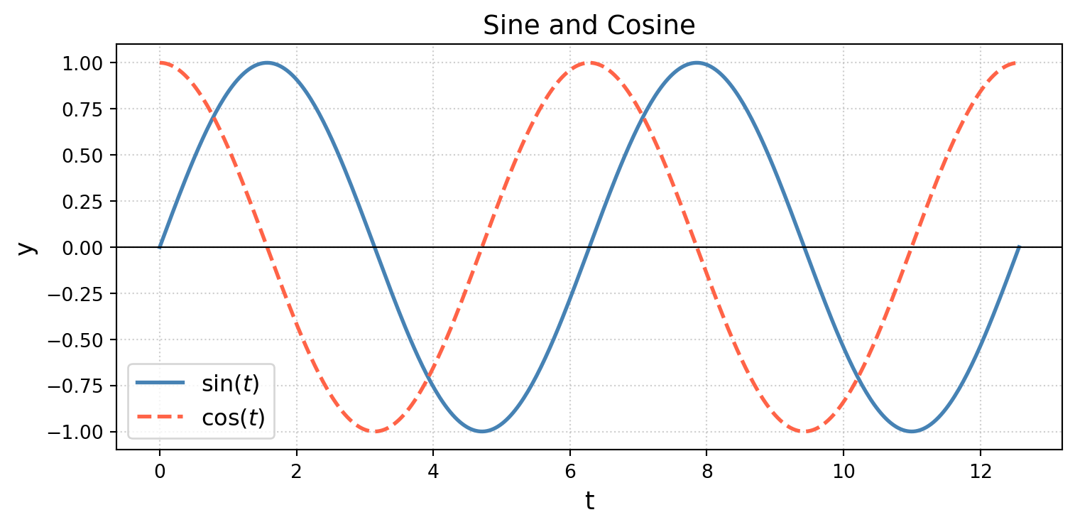

Key ideas:

fig, ax = plt.subplots() creates a figure (the whole image) and an axes (the plotting region). This is the recommended, object-oriented style.
ax.plot(x, y) draws a line.
LaTeX math can be used in labels by wrapping strings with r'$ ... $'.
plt.tight_layout() adjusts spacing to prevent clipped labels.

Plotting Multiple Subplots

fig, axes = plt.subplots(1, 2, figsize=(10, 4))   # 1 row, 2 columns

t = np.linspace(0, 4*np.pi, 400)

axes[0].plot(t, np.sin(t), color='steelblue', linewidth=2)
axes[0].set_title(r'$y = \sin(t)$')
axes[0].set_xlabel('t')
axes[0].grid(True, linestyle=':', alpha=0.6)

axes[1].plot(t, np.exp(-0.3 * t) * np.sin(t), color='tomato', linewidth=2)
axes[1].set_title(r'$y = e^{-0.3t}\sin(t)$')
axes[1].set_xlabel('t')
axes[1].grid(True, linestyle=':', alpha=0.6)

plt.tight_layout()
plt.show()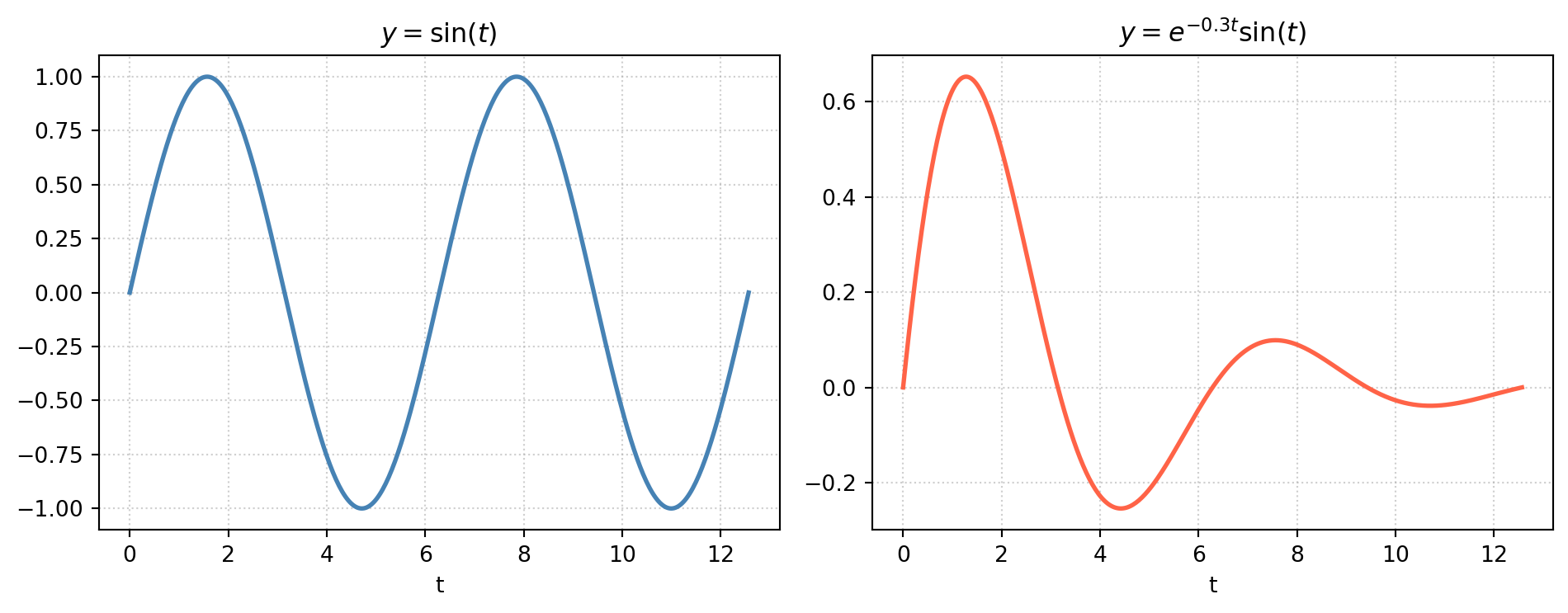

Saving Figures

fig.savefig("my_figure.png", dpi=150, bbox_inches="tight")
fig.savefig("my_figure.pdf")   # vector format; best for documents

Plotting Vector Fields

In the study of differential equations, direction fields (also called slope fields for first-order equations or vector fields for systems) are invaluable for understanding qualitative behavior.

Slope Field for a First-Order ODE

For $\dfrac{dy}{dt} = f(t, y)$, we draw a short line segment at each grid point $(t, y)$ with slope $f(t, y)$.

import matplotlib.pyplot as plt
import numpy as np

# ODE: dy/dt = t - y
def f(t, y):
    return t - y

# Create a grid of (t, y) values
t_vals = np.linspace(-1, 4, 20)
y_vals = np.linspace(-2, 5, 20)
T, Y = np.meshgrid(t_vals, y_vals)

# Compute slope at each grid point
dY = f(T, Y)
dT = np.ones_like(dY)            # dt component is always 1

# Normalize for uniform arrow length
magnitude = np.sqrt(dT**2 + dY**2)
dT_norm = dT / magnitude
dY_norm = dY / magnitude

fig, ax = plt.subplots(figsize=(7, 6))
ax.quiver(T, Y, dT_norm, dY_norm,
          angles='xy', color='steelblue', alpha=0.8, scale=25)

# Overlay a particular solution for reference
from scipy.integrate import solve_ivp
sol = solve_ivp(f, [-1, 4], [3.0], dense_output=True)
t_plot = np.linspace(-1, 4, 200)
ax.plot(t_plot, sol.sol(t_plot)[0], 'tomato', linewidth=2.5,
        label=r'Solution with $y(-1)=3$')

ax.set_xlabel('t', fontsize=13)
ax.set_ylabel('y', fontsize=13)
ax.set_title(r"Slope field: $\dfrac{dy}{dt} = t - y$", fontsize=14)
ax.legend(fontsize=12)
ax.set_xlim(-1, 4)
ax.set_ylim(-2, 5)
ax.grid(True, linestyle=':', alpha=0.5)
plt.tight_layout()
plt.show()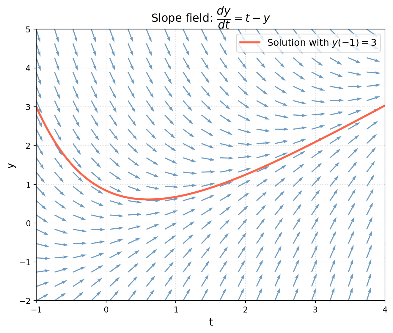

Vector Field for a 2 × 2 System

For the system $\dfrac{d\mathbf{x}}{dt} = A\mathbf{x}$, we draw arrows at each grid point $(x_1, x_2)$ pointing in the direction $(f_1, f_2)$.

# System: dx/dt = -x + y,  dy/dt = -x - y
def system(X, Y):
    dX = -X + Y
    dY = -X - Y
    return dX, dY

x_vals = np.linspace(-3, 3, 18)
y_vals = np.linspace(-3, 3, 18)
X, Y = np.meshgrid(x_vals, y_vals)
dX, dY = system(X, Y)

mag = np.sqrt(dX**2 + dY**2)
dX_n = dX / mag
dY_n = dY / mag

fig, ax = plt.subplots(figsize=(6, 6))
ax.quiver(X, Y, dX_n, dY_n, mag, cmap='coolwarm', alpha=0.9)
ax.set_xlabel(r'$x_1$', fontsize=13)
ax.set_ylabel(r'$x_2$', fontsize=13)
ax.set_title(r"Vector field: $\dot{x}_1 = -x_1+x_2,\;\dot{x}_2 = -x_1-x_2$",
             fontsize=12)
ax.set_aspect('equal')
ax.grid(True, linestyle=':', alpha=0.5)
plt.tight_layout()
plt.show()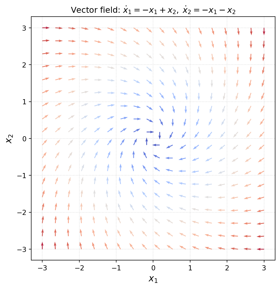

Tip

The cmap='coolwarm' coloring encodes the speed (magnitude) of the vector field — blue regions are slow, red regions are fast.

Intro to Scientific Python

Intro to NumPy

NumPy (Numerical Python) is the foundation of scientific computing in Python (Harris et al. 2020). Its central object is the ndarray — an efficient, multidimensional array.

Full documentation: https://numpy.org/doc/stable/

Creating Arrays

import numpy as np

# From a Python list
a = np.array([1, 2, 3, 4, 5])
print(a)          # [1 2 3 4 5]
print(a.dtype)    # int64  (data type)
print(a.shape)    # (5,)   (dimensions)

# Floating-point array
b = np.array([1.0, 2.0, 3.0])
print(b.dtype)    # float64

# 2-D array (matrix)
A = np.array([[1, 2, 3],
              [4, 5, 6]])
print(A.shape)    # (2, 3)  → 2 rows, 3 columns

[1 2 3 4 5]
int64
(5,)
float64
(2, 3)

Useful Array-Creation Functions

print(np.zeros(4))           # [0. 0. 0. 0.]
print(np.ones((2, 3)))       # 2×3 matrix of ones
print(np.eye(3))             # 3×3 identity matrix
print(np.linspace(0, 1, 5)) # [0.   0.25 0.5  0.75 1.  ]
print(np.arange(0, 10, 2))  # [0 2 4 6 8]

[0. 0. 0. 0.]
[[1. 1. 1.]
 [1. 1. 1.]]
[[1. 0. 0.]
 [0. 1. 0.]
 [0. 0. 1.]]
[0.   0.25 0.5  0.75 1.  ]
[0 2 4 6 8]

Array Arithmetic

NumPy operations act element-wise by default:

a = np.array([1.0, 2.0, 3.0])
b = np.array([4.0, 5.0, 6.0])

print(a + b)      # [5.  7.  9.]
print(a * b)      # [ 4. 10. 18.]  ← element-wise product
print(a ** 2)     # [1. 4. 9.]
print(np.sqrt(a)) # [1.    1.414 1.732]

[5. 7. 9.]
[ 4. 10. 18.]
[1. 4. 9.]
[1.         1.41421356 1.73205081]

Warning

a * b is not matrix multiplication. For matrix multiplication use A @ B or np.dot(A, B).

A = np.array([[1, 2], [3, 4]])
B = np.array([[5, 6], [7, 8]])
print(A @ B)       # matrix product

[[19 22]
 [43 50]]

Universal Functions (ufuncs)

NumPy provides vectorized versions of all standard math functions:

t = np.linspace(0, np.pi, 5)
print(np.sin(t))
print(np.exp(-t))
print(np.log(t + 1))

[0.00000000e+00 7.07106781e-01 1.00000000e+00 7.07106781e-01
 1.22464680e-16]
[1.         0.45593813 0.20787958 0.09478022 0.04321392]
[0.         0.57964145 0.94421571 1.21080774 1.42108041]

These are far faster than looping over elements manually.

Array Indexing and Slicing

a = np.array([10, 20, 30, 40, 50])
print(a[0])     # 10  (first element)
print(a[-1])    # 50  (last element)
print(a[1:4])   # [20 30 40]  (slice: indices 1,2,3)
print(a[::2])   # [10 30 50]  (every other element)

# 2-D indexing
A = np.arange(12).reshape(3, 4)
print(A)
print(A[1, 2])    # element in row 1, column 2
print(A[:, 1])    # all rows, column 1  (column vector)
print(A[0, :])    # row 0

10
50
[20 30 40]
[10 30 50]
[[ 0  1  2  3]
 [ 4  5  6  7]
 [ 8  9 10 11]]
6
[1 5 9]
[0 1 2 3]

Intro to SciPy

SciPy builds on NumPy and provides algorithms for optimization, integration, interpolation, signal processing, statistics, and — most importantly for us — differential equations (Virtanen et al. 2020).

Full documentation: https://docs.scipy.org/doc/scipy/

SciPy is organized into submodules:

Submodule	Content
`scipy.integrate`	Numerical integration, ODE solvers
`scipy.linalg`	Linear algebra
`scipy.optimize`	Root-finding, minimization
`scipy.signal`	Signal processing
`scipy.sparse`	Sparse matrices

Import submodules explicitly:

from scipy import integrate, linalg

SciPy’s ODE solvers and linear algebra routines are covered in the dedicated sections below.

Intro to SymPy

SymPy is a Python library for symbolic mathematics — it performs exact algebraic manipulations rather than numerical approximations (Meurer et al. 2017). Think of it as a free, Python-native computer algebra system (CAS).

Full documentation: https://docs.sympy.org/latest/

Symbols and Expressions

import sympy as sym

# Declare symbolic variables
t, y, C1, C2, k = sym.symbols('t y C1 C2 k', real=True)

# Build expressions
expr = sym.exp(-k * t) * sym.sin(t)
print(expr)

exp(-k*t)*sin(t)

Pretty Printing

sym.init_printing()   # enable pretty output in Jupyter/Quarto

expr2 = sym.sin(t)**2 + sym.cos(t)**2
print(sym.simplify(expr2))   # → 1

Calculus with SymPy

# Differentiation
f = sym.exp(-t) * sym.sin(2 * t)
df = sym.diff(f, t)
print("f'(t) =", df)

# Integration (indefinite)
integral = sym.integrate(f, t)
print("∫f dt =", integral)

# Definite integral
result = sym.integrate(sym.sin(t), (t, 0, sym.pi))
print("∫₀^π sin(t) dt =", result)   # 2

f'(t) = -exp(-t)*sin(2*t) + 2*exp(-t)*cos(2*t)
∫f dt = -exp(-t)*sin(2*t)/5 - 2*exp(-t)*cos(2*t)/5
∫₀^π sin(t) dt = 2

Solving Algebraic Equations

x = sym.Symbol('x')
solutions = sym.solve(x**2 - 5*x + 6, x)
print(solutions)   # [2, 3]

[2, 3]

Symbolic vs. Numerical

Feature	SymPy (symbolic)	NumPy/SciPy (numerical)
Results	Exact	Approximate (float)
Speed	Slower	Faster
Good for	Deriving formulas, exact solutions	Large-scale computation

You can convert a SymPy expression to a fast numerical function with sym.lambdify:

f_sym = sym.sin(t) * sym.exp(-t)
f_num = sym.lambdify(t, f_sym, modules='numpy')  # converts to NumPy function
t_vals = np.linspace(0, 5, 200)
y_vals = f_num(t_vals)   # fast NumPy evaluation
print(y_vals[:5])

[0.         0.02449962 0.04776835 0.06983789 0.09073981]

Numerical Methods for ODEs in Python

Using SciPy

scipy.integrate.solve_ivp is the primary tool for solving initial value problems (IVPs) numerically. It implements several Runge–Kutta and multi-step methods.

General call signature:

solve_ivp(fun, t_span, y0, method='RK45', t_eval=None, ...)

Argument	Meaning
`fun`	Function `f(t, y)` defining $y' = f(t,y)$
`t_span`	`(t0, tf)` — start and end times
`y0`	Initial condition (list or array)
`method`	ODE algorithm (default `'RK45'`)
`t_eval`	Times at which to store the solution

Example 1: First-Order Linear ODE

Solve $y' = -2y$, $y(0) = 3$, and compare with the exact solution $y(t) = 3e^{-2t}$.

from scipy.integrate import solve_ivp

def ode(t, y):
    """dy/dt = -2*y"""
    return [-2 * y[0]]          # must return a list/array

t_span = (0, 4)
y0 = [3.0]                      # initial condition as a list
t_eval = np.linspace(0, 4, 200) # times at which to record solution

sol = solve_ivp(ode, t_span, y0, method='RK45', t_eval=t_eval)

# sol.t  → time values
# sol.y  → array of shape (n_variables, n_times)

# Exact solution for comparison
y_exact = 3 * np.exp(-2 * sol.t)

fig, ax = plt.subplots(figsize=(7, 4))
ax.plot(sol.t, sol.y[0], 'steelblue', linewidth=2.5, label='RK45 (numerical)')
ax.plot(sol.t, y_exact,  'tomato',    linewidth=1.5, linestyle='--',
        label=r'Exact: $3e^{-2t}$')
ax.set_xlabel('t', fontsize=13)
ax.set_ylabel('y(t)', fontsize=13)
ax.set_title(r"$y' = -2y,\quad y(0)=3$", fontsize=14)
ax.legend(fontsize=12)
ax.grid(True, linestyle=':', alpha=0.6)
plt.tight_layout()
plt.show()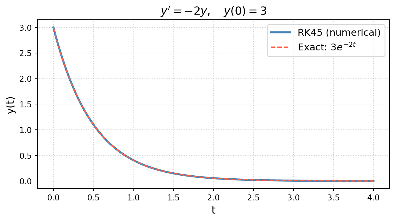

Example 2: Second-Order ODE (Mechanical Oscillator)

Solve the damped harmonic oscillator: $m x'' + c x' + k x = 0$.

We reduce to a first-order system: let $x_1 = x$, $x_2 = x'$. Then

\[x_1' = x_2, \qquad x_2' = -\frac{k}{m} x_1 - \frac{c}{m} x_2.\]

from scipy.integrate import solve_ivp

m = 1.0   # mass
c = 0.4   # damping coefficient
k = 5.0   # spring constant

def oscillator(t, state):
    """
    Damped harmonic oscillator as a first-order system.
    state = [x1, x2] = [position, velocity]
    """
    x1, x2 = state
    dx1 = x2
    dx2 = -(k/m) * x1 - (c/m) * x2
    return [dx1, dx2]

t_span = (0, 20)
y0     = [2.0, 0.0]         # initial position = 2, initial velocity = 0
t_eval = np.linspace(0, 20, 500)

sol = solve_ivp(oscillator, t_span, y0, method='RK45', t_eval=t_eval)

fig, ax = plt.subplots(figsize=(8, 4))
ax.plot(sol.t, sol.y[0], 'steelblue', linewidth=2, label='Position $x(t)$')
ax.plot(sol.t, sol.y[1], 'tomato',    linewidth=2, label='Velocity $x\'(t)$')
ax.set_xlabel('t', fontsize=13)
ax.set_ylabel('State', fontsize=13)
ax.set_title('Damped Harmonic Oscillator', fontsize=14)
ax.legend(fontsize=12)
ax.grid(True, linestyle=':', alpha=0.6)
plt.tight_layout()
plt.show()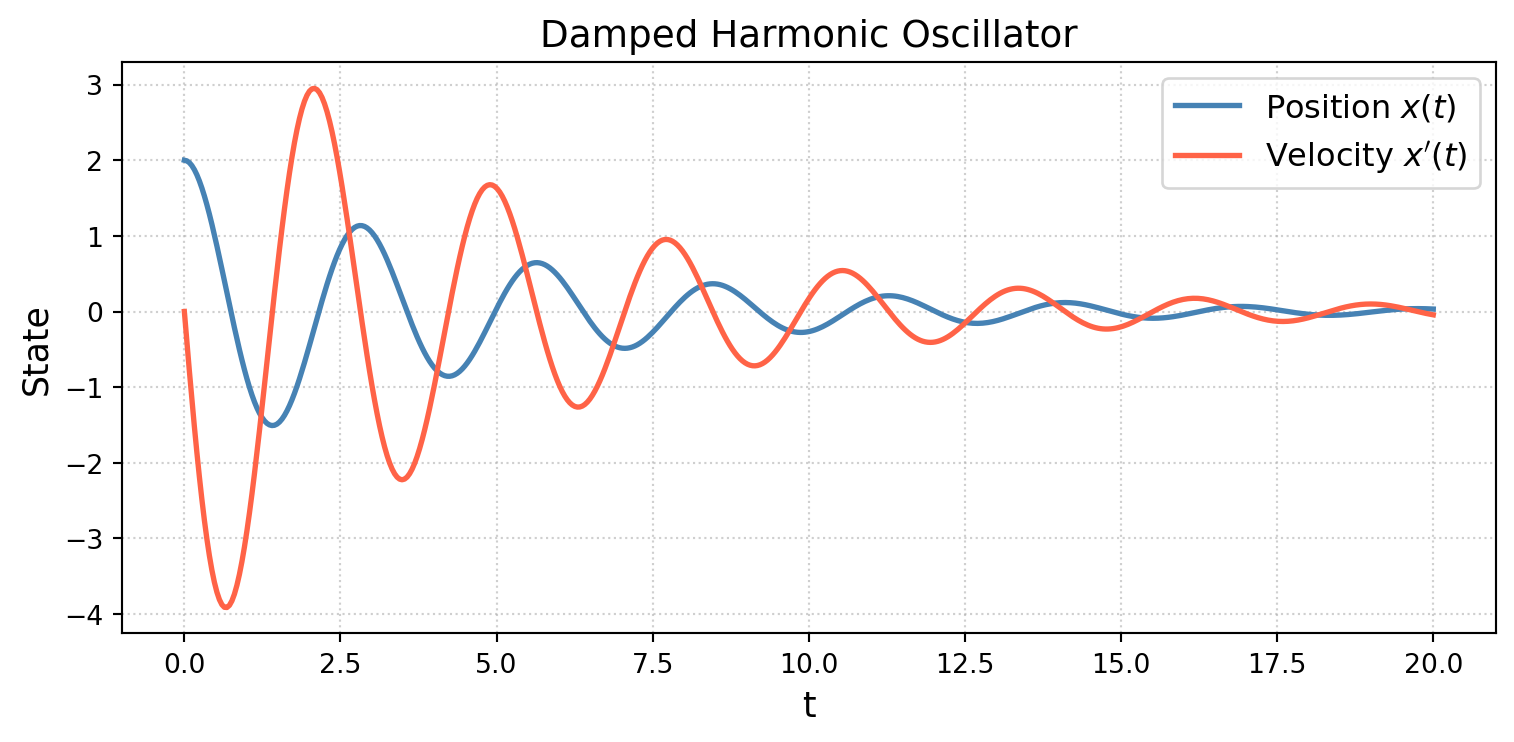

Example 3: Forced ODE

Solve $y'' + y = \cos(t)$ (resonance) with $y(0) = 0$, $y'(0) = 0$.

from scipy.integrate import solve_ivp

def forced_oscillator(t, state):
    x1, x2 = state
    dx1 = x2
    dx2 = -x1 + np.cos(t)   # forcing term cos(t) at natural frequency
    return [dx1, dx2]

t_span = (0, 40)
y0     = [0.0, 0.0]
t_eval = np.linspace(0, 40, 800)

sol = solve_ivp(forced_oscillator, t_span, y0, method='RK45', t_eval=t_eval,
                rtol=1e-8, atol=1e-10)   # tighter tolerances for accuracy

fig, ax = plt.subplots(figsize=(9, 4))
ax.plot(sol.t, sol.y[0], 'steelblue', linewidth=1.5)
ax.set_xlabel('t', fontsize=13)
ax.set_ylabel('y(t)', fontsize=13)
ax.set_title(r"Resonance: $y'' + y = \cos(t)$", fontsize=14)
ax.grid(True, linestyle=':', alpha=0.6)
plt.tight_layout()
plt.show()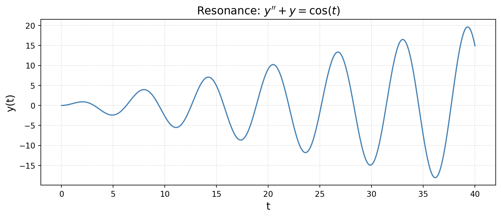

Available ODE Methods in `solve_ivp`

`method`	Description
`'RK45'`	Runge–Kutta 4(5); default; good for most problems
`'RK23'`	Runge–Kutta 2(3); lower accuracy, faster
`'DOP853'`	Dormand–Prince 8(5,3); high accuracy
`'Radau'`	Implicit Runge–Kutta; best for stiff problems
`'BDF'`	Backward differentiation formula; stiff problems
`'LSODA'`	Automatically detects stiffness

# Accessing the solution object
print("Success?", sol.success)
print("Message:", sol.message)
print("Solution shape (n_vars × n_times):", sol.y.shape)

Success? True
Message: The solver successfully reached the end of the integration interval.
Solution shape (n_vars × n_times): (2, 800)

Using SymPy

SymPy can find exact, closed-form solutions to ODEs when they exist.

import sympy as sym

t = sym.Symbol('t')
y = sym.Function('y')   # y is a function of t

Example 1: First-Order Linear ODE

Solve $y' + 2y = 4$, $y(0) = 1$.

ode_eq = sym.Eq(y(t).diff(t) + 2*y(t), 4)
general = sym.dsolve(ode_eq, y(t))
print("General solution:", general)

# Apply initial condition y(0) = 1
C1 = sym.Symbol('C1')
ic  = {C1: sym.solve(general.rhs.subs(t, 0) - 1, C1)[0]}
particular = general.subs(ic)
print("Particular solution:", particular)

General solution: Eq(y(t), C1*exp(-2*t) + 2)
Particular solution: Eq(y(t), 2 - exp(-2*t))

Example 2: Second-Order ODE

Solve $y'' - 3y' + 2y = 0$, $y(0) = 0$, $y'(0) = 1$.

ode2 = sym.Eq(y(t).diff(t,2) - 3*y(t).diff(t) + 2*y(t), 0)
general2 = sym.dsolve(ode2, y(t))
print("General solution:", general2)

C1, C2 = sym.symbols('C1 C2')
ics = sym.solve([
    general2.rhs.subs(t, 0) - 0,          # y(0) = 0
    general2.rhs.diff(t).subs(t, 0) - 1   # y'(0) = 1
], [C1, C2])
particular2 = general2.subs(ics)
print("Particular solution:", particular2)

General solution: Eq(y(t), (C1 + C2*exp(t))*exp(t))
Particular solution: Eq(y(t), (exp(t) - 1)*exp(t))

Example 3: Nonhomogeneous ODE

Solve $y'' + y = \sin(t)$ (the resonance equation) symbolically.

ode3 = sym.Eq(y(t).diff(t,2) + y(t), sym.sin(t))
general3 = sym.dsolve(ode3, y(t))
print(general3)

Eq(y(t), C2*sin(t) + (C1 - t/2)*cos(t))

Linear Algebra in Python

Numerical Linear Algebra with NumPy and SciPy

Matrices and Vectors

import numpy as np

A = np.array([[2, 1],
              [5, 3]], dtype=float)

b = np.array([4, 7], dtype=float)

print("Matrix A:\n", A)
print("Vector b:", b)

Matrix A:
 [[2. 1.]
 [5. 3.]]
Vector b: [4. 7.]

Solving Linear Systems $Ax = b$

from scipy import linalg

x = linalg.solve(A, b)
print("Solution x:", x)

# Verify: A @ x should equal b
print("Residual A @ x - b:", A @ x - b)

Solution x: [ 5. -6.]
Residual A @ x - b: [0.00000000e+00 3.55271368e-15]

Matrix Operations

# Transpose
print("A^T:\n", A.T)

# Determinant
print("det(A):", linalg.det(A))

# Inverse
print("A^{-1}:\n", linalg.inv(A))

# Matrix–vector product
print("A @ x:", A @ x)

# Matrix–matrix product
B = np.array([[1, 0], [0, 2]], dtype=float)
print("A @ B:\n", A @ B)

A^T:
 [[2. 5.]
 [1. 3.]]
det(A): 1.0
A^{-1}:
 [[ 3. -1.]
 [-5.  2.]]
A @ x: [4. 7.]
A @ B:
 [[2. 2.]
 [5. 6.]]

Computing Eigenvalues and Eigenvectors with NumPy and SciPy

For a square matrix $A$, the eigenvalue problem is $A\mathbf{v} = \lambda \mathbf{v}$.

import numpy as np
from scipy import linalg

A = np.array([[4, 1],
              [2, 3]], dtype=float)

# Using NumPy (returns unsorted eigenvalues)
eigenvalues, eigenvectors = np.linalg.eig(A)
print("Eigenvalues (NumPy):", eigenvalues)
print("Eigenvectors (columns):\n", eigenvectors)

Eigenvalues (NumPy): [5. 2.]
Eigenvectors (columns):
 [[ 0.70710678 -0.4472136 ]
 [ 0.70710678  0.89442719]]

# Using SciPy (more options; can return left eigenvectors, etc.)
vals, vecs = linalg.eig(A)
print("Eigenvalues (SciPy):", vals.real)

# The j-th eigenvector is vecs[:, j]
for j in range(len(vals)):
    lam = vals[j].real
    v   = vecs[:, j].real
    print(f"  λ = {lam:.4f},  v = {v}")
    print(f"  Verify A @ v = λ * v: {np.allclose(A @ v, lam * v)}")

Eigenvalues (SciPy): [5. 2.]
  λ = 5.0000,  v = [0.70710678 0.70710678]
  Verify A @ v = λ * v: True
  λ = 2.0000,  v = [-0.4472136   0.89442719]
  Verify A @ v = λ * v: True

Note

np.linalg.eig and scipy.linalg.eig may return complex eigenvalues even for real matrices (when complex eigenvalues occur in conjugate pairs). Use .real and .imag to extract real and imaginary parts.

# Symmetric matrices: use eigh for guaranteed real, sorted eigenvalues
C = np.array([[3, 1], [1, 2]], dtype=float)
vals_sym, vecs_sym = np.linalg.eigh(C)
print("Eigenvalues of symmetric matrix:", vals_sym)

Eigenvalues of symmetric matrix: [1.38196601 3.61803399]

Symbolic Linear Algebra with SymPy

import sympy as sym

A = sym.Matrix([[4, 1],
                [2, 3]])

print("Matrix A:")
sym.pprint(A)

# Determinant and inverse
print("\ndet(A) =", A.det())
print("\nA^{-1}:")
sym.pprint(A.inv())

Matrix A:
⎡4  1⎤
⎢    ⎥
⎣2  3⎦

det(A) = 10

A^{-1}:
⎡3/10  -1/10⎤
⎢           ⎥
⎣-1/5   2/5 ⎦

Solving Linear Systems Symbolically

b = sym.Matrix([5, 4])
x = A.solve(b)
print("Solution x:", x.T)

Solution x: Matrix([[11/10, 3/5]])

Computing Eigenvalues and Eigenvectors with SymPy

# eigenvals() returns {eigenvalue: algebraic_multiplicity, ...}
evals = A.eigenvals()
print("Eigenvalues:", evals)

# eigenvects() returns [(eigenvalue, multiplicity, [eigenvectors]), ...]
evects = A.eigenvects()
for lam, mult, vecs in evects:
    print(f"\nλ = {lam}  (multiplicity {mult})")
    for v in vecs:
        print(f"  eigenvector: {v.T}")

Eigenvalues: {5: 1, 2: 1}

λ = 2  (multiplicity 1)
  eigenvector: Matrix([[-1/2, 1]])

λ = 5  (multiplicity 1)
  eigenvector: Matrix([[1, 1]])

# Diagonalization: A = P * D * P^{-1}
P, D = A.diagonalize()
print("P ="); sym.pprint(P)
print("D ="); sym.pprint(D)
print("P * D * P^{-1} ="); sym.pprint(sym.simplify(P * D * P.inv()))

P =
⎡-1  1⎤
⎢     ⎥
⎣2   1⎦
D =
⎡2  0⎤
⎢    ⎥
⎣0  5⎦
P * D * P^{-1} =
⎡4  1⎤
⎢    ⎥
⎣2  3⎦

# Symbolic matrix with a parameter
a = sym.Symbol('a')
B = sym.Matrix([[a, 1], [1, a]])
print("Eigenvalues of [[a,1],[1,a]]:", B.eigenvals())

Eigenvalues of [[a,1],[1,a]]: {a - 1: 1, a + 1: 1}

Phase Portraits in Python

A phase portrait shows the trajectories of a two-dimensional autonomous system \[\frac{d\mathbf{x}}{dt} = \mathbf{f}(\mathbf{x}), \qquad \mathbf{x} = (x_1, x_2)^T,\] in the $(x_1, x_2)$ plane (the phase plane) for many different initial conditions.

from scipy.integrate import solve_ivp

def linear_system(t, state, A):
    """Linear system dx/dt = A*x."""
    return A @ np.array(state)

# System matrix
A_mat = np.array([[-1, 2],
                  [-2, -1]], dtype=float)

# Grid for the vector field
x1 = np.linspace(-3, 3, 18)
x2 = np.linspace(-3, 3, 18)
X1, X2 = np.meshgrid(x1, x2)
dX1 = A_mat[0, 0]*X1 + A_mat[0, 1]*X2
dX2 = A_mat[1, 0]*X1 + A_mat[1, 1]*X2
mag = np.sqrt(dX1**2 + dX2**2)

fig, ax = plt.subplots(figsize=(7, 7))

# Plot the vector field
ax.quiver(X1, X2, dX1/mag, dX2/mag, mag,
          cmap='Blues', alpha=0.7, scale=28)

# Plot several trajectories from different initial conditions
initial_conditions = [
    [2.5, 0], [-2.5, 0], [0, 2.5], [0, -2.5],
    [2, 2],   [-2, -2],  [2, -2],  [-2, 2]
]

t_span = (0, 6)
t_eval = np.linspace(0, 6, 300)

for ic in initial_conditions:
    sol = solve_ivp(linear_system, t_span, ic, args=(A_mat,),
                    t_eval=t_eval, method='RK45')
    ax.plot(sol.y[0], sol.y[1], 'tomato', linewidth=1.4, alpha=0.85)
    # Mark starting point
    ax.plot(ic[0], ic[1], 'ko', markersize=5)

ax.set_xlabel(r'$x_1$', fontsize=13)
ax.set_ylabel(r'$x_2$', fontsize=13)
ax.set_title(
    r'Phase portrait: $\dot{\mathbf{x}} = A\mathbf{x}$' +
    f'\n$A = [{A_mat[0,0]:.0f},{A_mat[0,1]:.0f};{A_mat[1,0]:.0f},{A_mat[1,1]:.0f}]$',
    fontsize=12
)
ax.axhline(0, color='k', linewidth=0.7)
ax.axvline(0, color='k', linewidth=0.7)
ax.set_aspect('equal')
ax.set_xlim(-3.2, 3.2)
ax.set_ylim(-3.2, 3.2)
ax.grid(True, linestyle=':', alpha=0.4)
plt.tight_layout()
plt.show()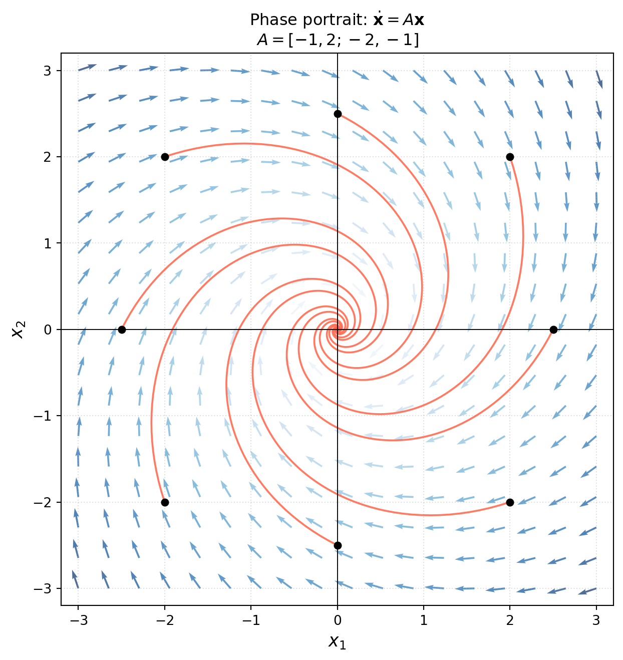

Nonlinear System: Pendulum

from scipy.integrate import solve_ivp

g = 9.8   # gravitational acceleration (m/s²)
L = 1.0   # pendulum length (m)

def pendulum(t, state):
    """
    Nonlinear pendulum (no damping).
    state = [theta, omega]  (angle, angular velocity)
    """
    theta, omega = state
    return [omega, -(g/L) * np.sin(theta)]

x1 = np.linspace(-np.pi, np.pi, 22)
x2 = np.linspace(-5, 5, 18)
X1, X2 = np.meshgrid(x1, x2)
dX1 = X2
dX2 = -(g/L) * np.sin(X1)
mag = np.sqrt(dX1**2 + dX2**2)

fig, ax = plt.subplots(figsize=(9, 6))
ax.quiver(X1, X2, dX1/mag, dX2/mag, mag, cmap='Blues', alpha=0.6, scale=28)

for theta0 in np.linspace(-2.8, 2.8, 9):
    for omega0 in [-3, -1, 0, 1, 3]:
        sol = solve_ivp(pendulum, (0, 8), [theta0, omega0],
                        t_eval=np.linspace(0, 8, 500), method='RK45',
                        rtol=1e-8, atol=1e-10)
        ax.plot(sol.y[0], sol.y[1], 'tomato', linewidth=0.9, alpha=0.7)

ax.set_xlabel(r'$\theta$ (rad)', fontsize=13)
ax.set_ylabel(r'$\omega$ (rad/s)', fontsize=13)
ax.set_title('Phase portrait: Nonlinear Pendulum', fontsize=14)
ax.set_xlim(-np.pi, np.pi)
ax.set_ylim(-5, 5)
ax.axhline(0, color='k', linewidth=0.7)
ax.grid(True, linestyle=':', alpha=0.4)
plt.tight_layout()
plt.show()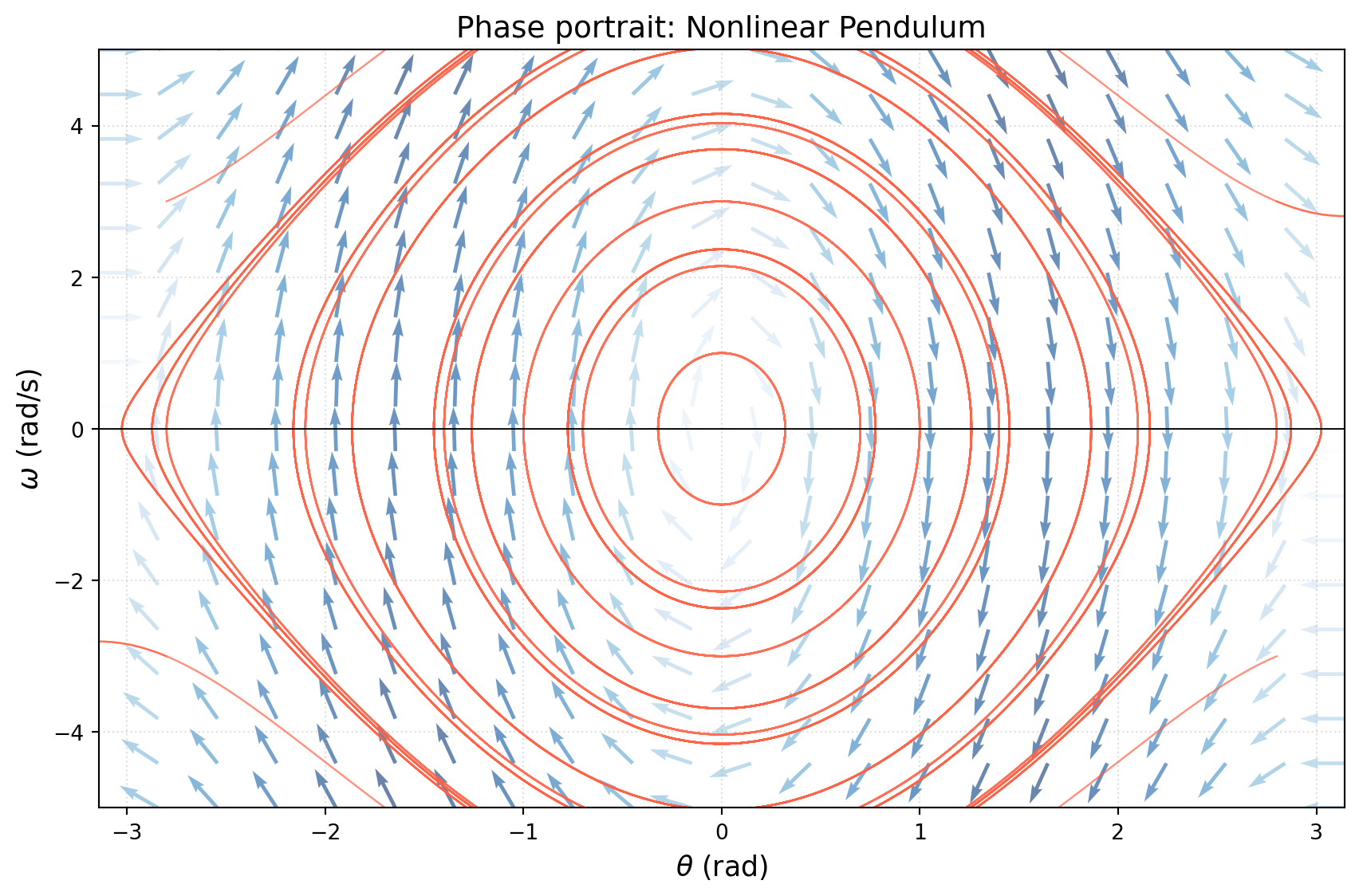

Laplace Transforms with SymPy

The Laplace transform $\mathcal{L}\{f(t)\}$ is an important tool for solving linear ODEs with constant coefficients. SymPy can compute Laplace transforms and inverse Laplace transforms symbolically.

import sympy as sym

t, s = sym.symbols('t s', positive=True)

# Forward Laplace transform
f = sym.exp(-2*t) * sym.sin(3*t)
F = sym.laplace_transform(f, t, s, noconds=True)
print("L{e^{-2t} sin(3t)} =", F)

L{e^{-2t} sin(3t)} = 3/((s + 2)**2 + 9)

# Inverse Laplace transform
G = s / (s**2 + 4)
g = sym.inverse_laplace_transform(G, s, t)
print("L^{-1}{s/(s²+4)} =", g)

L^{-1}{s/(s²+4)} = cos(2*t)

# Solving an IVP via Laplace transform
# Solve y'' + 4y = 0, y(0) = 1, y'(0) = 0

Y = sym.Function('Y')   # Y(s) = L{y(t)}

# Using known Laplace transform rules:
# L{y''} = s^2*Y - s*y(0) - y'(0)
#         = s^2*Y - s - 0
# So: (s^2 + 4)*Y = s  =>  Y = s/(s^2 + 4)
Y_s = s / (s**2 + 4)
y_t = sym.inverse_laplace_transform(Y_s, s, t)
print("Solution y(t) =", y_t)   # cos(2t)

Solution y(t) = cos(2*t)

Tips for Debugging Python Code

Even experienced programmers spend much of their time debugging. Here are some practical strategies.

Read the Error Message

Python’s error messages are informative. The last line tells you the error type and a short description; the lines above show the traceback — where in the code the error occurred.

# Common error types
# NameError    — you used a variable or function that isn't defined
# TypeError    — wrong type passed to a function
# ValueError   — right type, but inappropriate value
# IndexError   — index out of bounds
# ZeroDivisionError — division by zero
# AttributeError — object doesn't have the attribute/method you called

Use `print` Statements

Insert print() calls to inspect intermediate values:

def my_ode(t, y):
    result = -2 * y[0]
    print(f"t={t:.3f}, y={y[0]:.6f}, f={result:.6f}")  # debug line
    return [result]

Check Array Shapes

Shape mismatches are a common source of errors in NumPy code:

print(A.shape)   # always check shapes when something looks wrong
print(b.shape)

Useful Resources

Official Python Docs
Stack Overflow — searching your exact error message often finds an answer immediately
NumPy Debugging Guide

References

Harris, Charles R., K. Jarrod Millman, Stéfan J. van der Walt, et al. 2020. “Array Programming with NumPy.” Nature 585: 357–62. https://doi.org/10.1038/s41586-020-2649-2.

Hunter, John D. 2007. “Matplotlib: A 2D Graphics Environment.” Computing in Science & Engineering 9 (3): 90–95. https://doi.org/10.1109/MCSE.2007.55.

Meurer, Aaron, Christopher P. Smith, Mateusz Paprocki, et al. 2017. “SymPy: Symbolic Computing in Python.” PeerJ Computer Science 3: e103. https://doi.org/10.7717/peerj-cs.103.

Python Software Foundation. 2024. Python Language Reference, Version 3. https://docs.python.org/3/.

Virtanen, Pauli, Ralf Gommers, Travis E. Oliphant, et al. 2020. “SciPy 1.0: Fundamental Algorithms for Scientific Computing in Python.” Nature Methods 17: 261–72. https://doi.org/10.1038/s41592-019-0686-2.

Expand for Session Info

Show the code

import sys
print("Python version:", sys.version)
print('\n'.join(f'{m.__name__}=={m.__version__}' for m in globals().values() if getattr(m, '__version__', None)))

Python version: 3.14.4 | packaged by conda-forge | (main, Apr  8 2026, 02:33:53) [Clang 20.1.8 ]
numpy==2.4.3
scipy==1.17.1
sympy==1.14.0
matplotlib==3.10.8

Reuse

CC BY-NC-SA 4.0

Installing and Managing Python and Packages

Option 1: uv (Recommended for New Users)

Option 2: conda / Anaconda

Choosing an Editor / Interface

Overview of Python and Python Modules

What is Python?

What is a Python Module (Package)?

Importing Modules and Namespaces

Writing Functions

Basic Function Syntax

Functions with Multiple Arguments and Default Values

Lambda Functions (Anonymous Functions)

Returning Multiple Values

Plotting

Basic Plotting

Plotting Multiple Subplots

Saving Figures

Plotting Vector Fields

Slope Field for a First-Order ODE

Vector Field for a 2 × 2 System

Intro to Scientific Python

Intro to NumPy

Creating Arrays

Useful Array-Creation Functions

Array Arithmetic

Universal Functions (ufuncs)

Array Indexing and Slicing

Intro to SciPy

Intro to SymPy

Symbols and Expressions

Pretty Printing

Calculus with SymPy

Solving Algebraic Equations

Symbolic vs. Numerical

Numerical Methods for ODEs in Python

Using SciPy

Example 1: First-Order Linear ODE

Example 2: Second-Order ODE (Mechanical Oscillator)

Example 3: Forced ODE

Available ODE Methods in solve_ivp

Using SymPy

Example 1: First-Order Linear ODE

Example 2: Second-Order ODE

Example 3: Nonhomogeneous ODE

Linear Algebra in Python

Numerical Linear Algebra with NumPy and SciPy

Matrices and Vectors

Solving Linear Systems \(Ax = b\)

Matrix Operations

Computing Eigenvalues and Eigenvectors with NumPy and SciPy

Symbolic Linear Algebra with SymPy

Solving Linear Systems Symbolically

Computing Eigenvalues and Eigenvectors with SymPy

Phase Portraits in Python

Nonlinear System: Pendulum

Laplace Transforms with SymPy

Tips for Debugging Python Code

Read the Error Message

Use print Statements

Check Array Shapes

Useful Resources

References

Reuse

Option 1: `uv` (Recommended for New Users)

Option 2: `conda` / Anaconda

Available ODE Methods in `solve_ivp`

Use `print` Statements