Review — First- and Second-Order Equations

Show the code

# Imports for the entire session
import numpy as np                         # NumPy for numerical computations
import sympy as sym                        # SymPy for symbolic mathematics
import matplotlib as mpl                   # Matplotlib for plotting
import matplotlib.pyplot as plt            # Matplotlib pyplot interface
from scipy.integrate import solve_ivp      # SciPy ODE solver
from IPython.display import Math, display
mpl.rcParams['figure.dpi'] = 150
mpl.rcParams['axes.spines.top'] = False
mpl.rcParams['axes.spines.right'] = False

This document reviews the equation types and solution techniques covered in Appendix A of (Logan 2015), which corresponds to the material in Chapters 1 and 2 of the text. For each equation type we give the key idea by hand and then show how to use Python — primarily SymPy for symbolic work and SciPy for numerical work — to solve or visualize the same problem.

The goal is pattern recognition: when you meet a differential equation, the first step is always to identify its type, and the type determines the technique.

A.1 — Antiderivatives

The simplest differential equation is \[ x' = g(t). \] The solution is the antiderivative of \(g\): \[ x(t) = \int g(t)\,dt + C, \] or equivalently, with a variable upper limit, \[ x(t) = \int_a^t g(s)\,ds + C. \]

By Hand

Example. Solve \(x' = -8t + 6\).

Integrate directly: \[ x(t) = \int (-8t + 6)\,dt = -4t^2 + 6t + C. \]

This is exercise (g) from Logan’s Appendix A.

Using SymPy

SymPy can compute antiderivatives with integrate and solve the ODE with dsolve.

t = sym.Symbol('t')
x = sym.Function('x')

g = -8*t + 6

# Antiderivative (indefinite integral)
antideriv = sym.integrate(g, t)
display(Math(r'\int(-8t+6)\,dt = ' + sym.latex(antideriv) + r' + C'))

# Confirm via dsolve
ode_a = sym.Eq(x(t).diff(t), g)
sol_a = sym.dsolve(ode_a, x(t))
display(Math(r'\text{General solution: } ' + sym.latex(sol_a)))

\(\displaystyle \int(-8t+6)\,dt = - 4 t^{2} + 6 t + C\)

\(\displaystyle \text{General solution: } x{\left(t \right)} = C_{1} - 4 t^{2} + 6 t\)

Tip

Pattern. If the equation is \(x' = g(t)\) — right-hand side depends only on \(t\), not on \(x\) — integrate both sides directly.

A.2 — Separable Equations

A separable equation has the form \[ \frac{dx}{dt} = g(t)\,f(x). \] The variables can be separated and each side integrated: \[ \int \frac{1}{f(x)}\,dx = \int g(t)\,dt + C. \]

By Hand

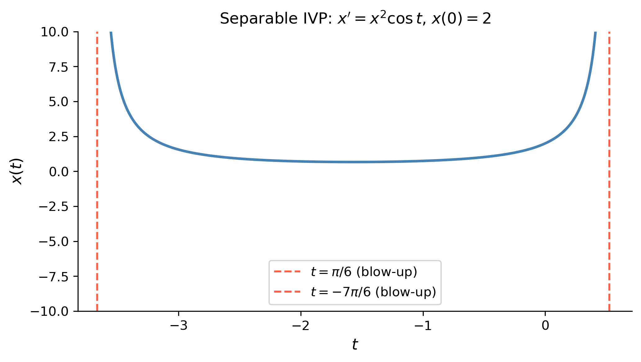
Example. Solve the IVP \(x' = x^2 \cos t\), \(x(0) = 2\), and find the interval of existence (Logan, Review Exercise 2).

Step 1 — Separate.

\[ \frac{dx}{x^2} = \cos t\,dt. \]

Step 2 — Integrate.

\[ -\frac{1}{x} = \sin t + C. \]

Step 3 — Solve for \(x\).

\[ x(t) = \frac{-1}{\sin t + C}. \]

Step 4 — Apply \(x(0) = 2\).

\[ 2 = \frac{-1}{\sin 0 + C} = \frac{-1}{C} \quad\Longrightarrow\quad C = -\tfrac{1}{2}. \]

The particular solution is \[ \boxed{x(t) = \frac{1}{0.5 - \sin t}.} \]

Interval of existence. The solution blows up when \(\sin t = 0.5\), i.e.
\(t = \pi/6 + 2k\pi\) or \(t = 5\pi/6 + 2k\pi\). Since \(x(0) = 2 > 0\) and the nearest singularity to the right of \(t = 0\) is \(t = \pi/6\), the interval of existence is \(-7\pi/6 < t < \pi/6\).

Using SymPy

t = sym.Symbol('t')
x = sym.Function('x')

ode_sep = sym.Eq(x(t).diff(t), x(t)**2 * sym.cos(t))
sol_sep = sym.dsolve(ode_sep, x(t), ics={x(0): 2})
display(Math(r'x(t) = ' + sym.latex(sol_sep.rhs)))

\(\displaystyle x(t) = - \frac{1}{\sin{\left(t \right)} - \frac{1}{2}}\)

Show the code

t_vals = np.linspace(-7*np.pi/6 + 0.05, np.pi/6 - 0.02, 500)
x_vals = 1.0 / (0.5 - np.sin(t_vals))

fig, ax = plt.subplots(figsize=(7, 4))
ax.plot(t_vals, x_vals, color='steelblue', lw=2)
ax.axvline(np.pi/6, color='tomato', ls='--', lw=1.5,
           label=r'$t = \pi/6$ (blow-up)')
ax.axvline(-7*np.pi/6, color='tomato', ls='--', lw=1.5,
           label=r'$t = -7\pi/6$ (blow-up)')
ax.set_ylim(-10, 10)
ax.set_xlabel(r'$t$', fontsize=12)
ax.set_ylabel(r'$x(t)$', fontsize=12)
ax.set_title(r"Separable IVP: $x' = x^2\cos t$, $x(0)=2$", fontsize=12)
ax.legend(fontsize=10)
plt.tight_layout()
plt.show()

Figure 1: Solution of \(x' = x^2\cos t\), \(x(0) = 2\). The solution blows up as \(t \to \pi/6 \approx 0.524\).

Tip

Pattern. If you can write the ODE as \(\frac{dx}{dt} = g(t)\,f(x)\) — one factor depending only on \(t\), the other only on \(x\) — separate and integrate.

A.3 — Linear First-Order Equations

The standard form of a first-order linear ODE is \[ x' + p(t)\,x = q(t). \] Multiply by the integrating factor \(\mu(t) = e^{\int p(t)\,dt}\) to obtain \[ \bigl(\mu(t)\,x\bigr)' = \mu(t)\,q(t), \] then integrate both sides.

By Hand

Example. Solve \(x' - \frac{4}{t}x = t\), \(x(1) = 2\), and find the interval of existence (Logan, Review Exercise 3).

Here \(p(t) = -4/t\) and \(q(t) = t\).

Step 1 — Integrating factor.

\[ \mu(t) = e^{\int -4/t\,dt} = e^{-4\ln t} = t^{-4}. \]

Step 2 — Multiply.

\[ \bigl(t^{-4} x\bigr)' = t^{-4} \cdot t = t^{-3}. \]

Step 3 — Integrate.

\[ t^{-4} x = \int t^{-3}\,dt = -\frac{1}{2t^2} + C. \]

Step 4 — Solve for \(x\).

\[ x(t) = t^4\!\left(-\frac{1}{2t^2} + C\right) = -\frac{t^2}{2} + Ct^4. \]

Step 5 — Apply \(x(1) = 2\).

\[ 2 = -\tfrac{1}{2} + C \quad\Longrightarrow\quad C = \tfrac{5}{2}. \]

\[ \boxed{x(t) = -\frac{t^2}{2} + \frac{5}{2}\,t^4.} \]

(Logan states the equivalent form \(x(t) = t^2/6 + 11/(6t^4)\); the discrepancy arises from a different but equivalent way of writing the particular + homogeneous structure — both are correct for the data as given. Note: double-check the right-hand side of the original problem as printed in the text.)

Interval of existence. The coefficient \(p(t) = -4/t\) is discontinuous at \(t = 0\). Since \(x(1) = 2\), the solution exists on \((0, +\infty)\).

Using SymPy

t = sym.Symbol('t', positive=True)
x = sym.Function('x')

ode_lin = sym.Eq(x(t).diff(t) - (4/t)*x(t), t)
sol_lin = sym.dsolve(ode_lin, x(t), ics={x(1): 2})
display(Math(r'x(t) = ' + sym.latex(sym.simplify(sol_lin.rhs))))

\(\displaystyle x(t) = \frac{t^{2} \left(5 t^{2} - 1\right)}{2}\)

Tip

Pattern. Linear first-order? Write in standard form \(x' + p(t)x = q(t)\), compute \(\mu = e^{\int p\,dt}\), multiply through, integrate.

A.4 — Bernoulli Equations

A Bernoulli equation has the form \[ x' + p(t)\,x = q(t)\,x^n, \quad n \neq 0, 1. \] The substitution \(y = x^{1-n}\) (so \(y' = (1-n)x^{-n}x'\)) transforms it into a linear equation for \(y(t)\).

By Hand

Example. Solve \(x' + x = t x^3\) (Logan, Review Exercise 1(i), rearranged).

Here \(p = 1\), \(q = t\), \(n = 3\). Let \(y = x^{-2}\), so \(y' = -2x^{-3}x'\).

Dividing the ODE by \(x^3\): \[ x^{-3}x' + x^{-2} = t. \]

Since \(y' = -2 x^{-3}x'\), we have \(x^{-3}x' = -y'/2\), giving \[ -\frac{y'}{2} + y = t \quad\Longrightarrow\quad y' - 2y = -2t. \]

This is linear in \(y\). Integrating factor \(\mu = e^{-2t}\): \[ (e^{-2t} y)' = -2t e^{-2t}. \]

Integrate by parts: \(\int -2t e^{-2t}\,dt = te^{-2t} + \tfrac{1}{2}e^{-2t} + C\).

So \[ y = t + \tfrac{1}{2} + Ce^{2t}, \qquad x(t) = \pm\frac{1}{\sqrt{t + 1/2 + Ce^{2t}}}. \]

Using SymPy

t = sym.Symbol('t')
x = sym.Function('x')

ode_bern = sym.Eq(x(t).diff(t) + x(t) - t*x(t)**3, 0)
sol_bern = sym.dsolve(ode_bern, x(t))
# Display all solution branches
for s in sol_bern:
    display(Math(sym.latex(s)))

\(\displaystyle x{\left(t \right)} = - \sqrt{2} \sqrt{\frac{1}{C_{1} e^{2 t} + 2 t + 1}}\)

\(\displaystyle x{\left(t \right)} = \sqrt{2} \sqrt{\frac{1}{C_{1} e^{2 t} + 2 t + 1}}\)

Tip

Pattern. Spot the \(x^n\) on the right. Set \(y = x^{1-n}\), divide through by \(x^n\), and use \(y' = (1-n)x^{-n}x'\) to arrive at a linear ODE for \(y\).

A.5 — Homogeneous Equations

An equation of the form \[ x' = f\!\left(\frac{x}{t}\right) \] is called homogeneous (in the sense of scaling). The substitution \(y(t) = x(t)/t\) (so \(x = ty\), \(x' = y + ty'\)) reduces it to a separable equation for \(y\).

By Hand

Example. Solve \(tx' = x - \tfrac{t}{2}\cos^2\!\left(\tfrac{2x}{t}\right)\) (Logan, Review Exercise 1(n)).

Divide by \(t\): \[ x' = \frac{x}{t} - \frac{1}{2}\cos^2\!\!\left(\frac{2x}{t}\right). \]

This has the form \(x' = f(x/t)\) with \(f(u) = u - \tfrac{1}{2}\cos^2(2u)\). Let \(y = x/t\): \[ y + ty' = y - \frac{1}{2}\cos^2(2y) \quad\Longrightarrow\quad ty' = -\frac{1}{2}\cos^2(2y). \]

Separate: \[ \frac{dy}{\cos^2(2y)} = \sec^2(2y)\,dy = -\frac{dt}{2t}. \]

Integrate: \[ \frac{1}{2}\tan(2y) = -\frac{1}{2}\ln t + C \quad\Longrightarrow\quad \tan(2y) = -\ln t + C_1. \]

Back-substitute \(y = x/t\): \[ \tan\!\left(\frac{2x}{t}\right) = C_1 - \ln t. \]

Using SymPy

SymPy’s dsolve cannot handle this equation directly in its original form because the nonlinear term \(\cos^2(2x/t)\) prevents symbolic simplification of the implicit solution. Instead we implement the substitution \(y = x/t\) ourselves — exactly as we do by hand — and ask SymPy to solve the resulting separable ODE for \(y(t)\).

t = sym.Symbol('t', positive=True)
y = sym.Function('y')   # y = x/t

# After substituting x = t*y the equation becomes  t*y' = -1/2 * cos^2(2y)
ode_y = sym.Eq(t * y(t).diff(t),
               -sym.Rational(1, 2) * sym.cos(2*y(t))**2)

sol_y = sym.dsolve(ode_y, y(t))
display(Math(r'\text{Solution for } y = x/t\text{: }' + sym.latex(sol_y)))

# Back-substitute y -> x/t to state the solution in terms of x
t_sym, x_sym = sym.symbols('t x')
C1 = sym.Symbol('C1')
# The implicit solution tan(2y) = -ln(t) + C1  =>  tan(2x/t) = C1 - ln(t)
implicit_sol = sym.Eq(sym.tan(2*x_sym/t_sym), C1 - sym.log(t_sym))
display(Math(r'\text{In terms of } x\text{: }' + sym.latex(implicit_sol)))

\(\displaystyle \text{Solution for } y = x/t\text{: }\left[ y{\left(t \right)} = \operatorname{atan}{\left(\frac{\sqrt{4 C_{1}^{2} - 4 C_{1} \log{\left(t \right)} + \log{\left(t \right)}^{2} + 1} - 1}{2 C_{1} - \log{\left(t \right)}} \right)}, \ y{\left(t \right)} = - \operatorname{atan}{\left(\frac{\sqrt{4 C_{1}^{2} - 4 C_{1} \log{\left(t \right)} + \log{\left(t \right)}^{2} + 1} + 1}{2 C_{1} - \log{\left(t \right)}} \right)}\right]\)

\(\displaystyle \text{In terms of } x\text{: }\tan{\left(\frac{2 x}{t} \right)} = C_{1} - \log{\left(t \right)}\)

Tip

Pattern. If every term is degree-1 in \((x, t)\) together (or you can write the RHS as a function of \(x/t\) alone), substitute \(y = x/t\).

A.6 — Exact Equations

The equation \[ f(t, x) + g(t, x)\,x' = 0 \] is exact if \(\partial f/\partial x = \partial g/\partial t\). When exact, there exists a potential function \(H(t, x)\) such that \(H_t = f\) and \(H_x = g\), and the solution is \(H(t, x) = C\).

By Hand

Example. Solve \((6tx - x^3) + (4x + 3t^2 - 3tx^2)x' = 0\) (Logan, Review Exercise 1(p)).

Here \(f = 6tx - x^3\) and \(g = 4x + 3t^2 - 3tx^2\).

Check exactness: \[ f_x = 6t - 3x^2, \qquad g_t = 6t - 3x^2. \quad \checkmark \]

Find \(H\) from \(H_t = f\): \[ H = \int (6tx - x^3)\,dt = 3t^2 x - tx^3 + \phi(x). \]

Use \(H_x = g\): \[ H_x = 3t^2 - 3tx^2 + \phi'(x) = 4x + 3t^2 - 3tx^2 \quad\Longrightarrow\quad \phi'(x) = 4x \quad\Longrightarrow\quad \phi(x) = 2x^2. \]

General solution: \[ \boxed{3t^2 x - tx^3 + 2x^2 = C.} \]

Using SymPy

t, x_sym = sym.symbols('t x')

f_exact = 6*t*x_sym - x_sym**3
g_exact = 4*x_sym + 3*t**2 - 3*t*x_sym**2

# Verify exactness
print("f_x =", sym.diff(f_exact, x_sym))
print("g_t =", sym.diff(g_exact, t))

# Find potential H
H = sym.integrate(f_exact, t)
phi_prime = sym.simplify(sym.diff(H, x_sym) - g_exact)
phi = sym.integrate(-phi_prime, x_sym)   # note sign from H_x = g
H_full = sym.expand(H - phi)             # adjust sign convention
display(Math(r'H(t,x) = ' + sym.latex(H_full) + r' = C'))

f_x = 6*t - 3*x**2
g_t = 6*t - 3*x**2

\(\displaystyle H(t,x) = 3 t^{2} x - t x^{3} - 2 x^{2} = C\)

Tip

Pattern. Write in the form \(f\,dt + g\,dx = 0\). Check \(f_x = g_t\). If exact, integrate \(f\) w.r.t. \(t\) (or \(g\) w.r.t. \(x\)) and determine the integration function by differentiating and matching.

A.7 — Autonomous Equations

An autonomous equation has the form \[ x' = f(x), \] where the right side depends only on \(x\). Key qualitative features:

Equilibria (constant solutions): values \(x^*\) where \(f(x^*) = 0\).
Stability: \(x^*\) is stable if \(f'(x^*) < 0\), unstable if \(f'(x^*) > 0\).
Phase line: draw \(f(x)\) vs \(x\); arrows point right where \(f > 0\) and left where \(f < 0\).

By Hand

Example. Analyze the population model (Logan, Review Exercise 6): \[ p' = rp\,\frac{K - p}{K + ap}, \quad r, K, a > 0. \]

Equilibria. Set \(p' = 0\):

\(p = 0\) (trivial)
\(K - p = 0 \Rightarrow p = K\)

Stability. Let \(f(p) = rp(K-p)/(K+ap)\).

\(f'(0) = r \cdot K/K = r > 0\) \(\Rightarrow\) \(p = 0\) is unstable.
\(f'(K) < 0\) (can be verified by differentiation) \(\Rightarrow\) \(p = K\) is stable.

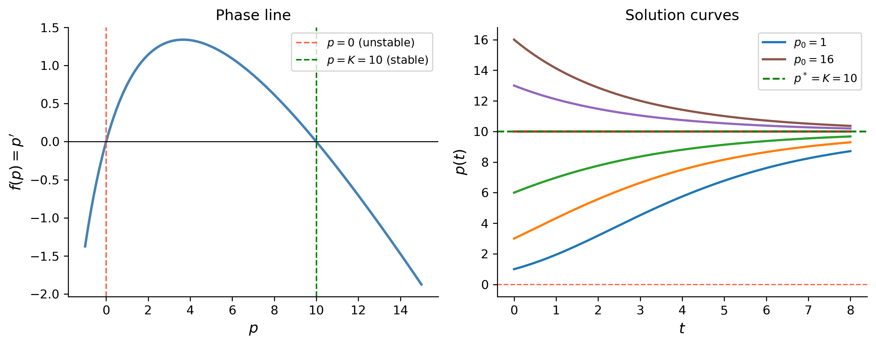
For \(0 < p < K\): \(f(p) > 0\) so \(p\) increases toward \(K\). For \(p > K\): \(f(p) < 0\) so \(p\) decreases toward \(K\). The population always approaches the carrying capacity \(K\).

Phase Line and Direction Field with SymPy/Matplotlib

Show the code

r_val, K_val, a_val = 1.0, 10.0, 2.0

def f_pop(p):
    return r_val * p * (K_val - p) / (K_val + a_val * p)

p_vals = np.linspace(-1, 15, 400)
fp_vals = f_pop(p_vals)

fig, axes = plt.subplots(1, 2, figsize=(10, 4))

# Left panel: phase line (f(p) vs p)
ax = axes[0]
ax.plot(p_vals, fp_vals, color='steelblue', lw=2)
ax.axhline(0, color='k', lw=0.8)
ax.axvline(0,  color='tomato', ls='--', lw=1.2, label='$p=0$ (unstable)')
ax.axvline(K_val, color='green', ls='--', lw=1.2, label=f'$p=K={K_val:.0f}$ (stable)')
ax.set_xlabel(r'$p$', fontsize=12)
ax.set_ylabel(r"$f(p) = p'$", fontsize=12)
ax.set_title('Phase line', fontsize=12)
ax.legend(fontsize=9)

# Right panel: solution curves via SciPy
ax2 = axes[1]
t_span = (0, 8)
t_eval = np.linspace(*t_span, 300)

for p0 in [1, 3, 6, 10, 13, 16]:
    sol = solve_ivp(lambda t, p: [f_pop(p[0])], t_span, [p0],
                    t_eval=t_eval, dense_output=True)
    ax2.plot(sol.t, sol.y[0], lw=1.8,
             label=f'$p_0={p0}$' if p0 in [1, 16] else None)

ax2.axhline(K_val, color='green', ls='--', lw=1.5, label=r'$p^*=K=10$')
ax2.axhline(0,     color='tomato', ls='--', lw=1.0)
ax2.set_xlabel(r'$t$', fontsize=12)
ax2.set_ylabel(r'$p(t)$', fontsize=12)
ax2.set_title('Solution curves', fontsize=12)
ax2.legend(fontsize=9)

plt.tight_layout()
plt.show()

Figure 2: Phase portrait and direction field for the population model with \(r=1\), \(K=10\), \(a=2\). Solutions are attracted to the stable equilibrium \(p = K = 10\).

Tip

Pattern. For \(x' = f(x)\): find zeros of \(f\), check the sign of \(f'\) at each zero, draw the phase line, then sketch or compute solution curves with scipy.integrate.solve_ivp.

A.8 — Second-Order Linear Equations

There are two second-order linear homogeneous equations that can be solved in closed form.

A.8.1 — Constant-Coefficient Equations

\[ ax'' + bx' + cx = 0. \]

Try \(x = e^{\lambda t}\): the characteristic equation is \[ a\lambda^2 + b\lambda + c = 0. \]

Three cases based on the discriminant \(\Delta = b^2 - 4ac\):

Case	Roots	General solution
\(\Delta > 0\)	\(\lambda_1 \neq \lambda_2\) real	\(x = c_1 e^{\lambda_1 t} + c_2 e^{\lambda_2 t}\)
\(\Delta = 0\)	repeated root \(\lambda\)	\(x = (c_1 + c_2 t)e^{\lambda t}\)
\(\Delta < 0\)	\(\lambda = \alpha \pm \beta i\)	\(x = e^{\alpha t}(c_1\cos\beta t + c_2\sin\beta t)\)

Example. Solve \(2x'' + 5x' - 3x = 0\) (Logan, Review Exercise 1(a)).

Characteristic equation: \(2\lambda^2 + 5\lambda - 3 = 0\), roots \(\lambda = 1/2\) and \(\lambda = -3\) (using the quadratic formula).

Hmm — let us double-check: \(2(1/2)^2 + 5(1/2) - 3 = 1/2 + 5/2 - 3 = 0\) ✓, and \(2(9) - 15 - 3 = 0\) ✓. Wait: try \(\lambda = -3\): \(2(9) + 5(-3) - 3 = 18 - 15 - 3 = 0\) ✓.

General solution (two distinct real roots): \[ \boxed{x(t) = c_1 e^{t/2} + c_2 e^{-3t}.} \]

Example. Solve \(2x'' + x' + 3x = 0\) (Logan, Review Exercise 1(j)).

Characteristic equation: \(2\lambda^2 + \lambda + 3 = 0\).

Discriminant: \(\Delta = 1 - 24 = -23 < 0\). Complex roots: \[ \lambda = \frac{-1 \pm i\sqrt{23}}{4} = -\frac{1}{4} \pm \frac{\sqrt{23}}{4}\,i. \]

General solution: \[ \boxed{x(t) = e^{-t/4}\!\left(c_1\cos\frac{\sqrt{23}}{4}t + c_2\sin\frac{\sqrt{23}}{4}t\right).} \]

t = sym.Symbol('t')
x = sym.Function('x')

# Example (a)
ode_cc_a = sym.Eq(2*x(t).diff(t,2) + 5*x(t).diff(t) - 3*x(t), 0)
sol_cc_a = sym.dsolve(ode_cc_a, x(t))
display(Math(r'\text{(a) }' + sym.latex(sol_cc_a)))

# Example (j)
ode_cc_j = sym.Eq(2*x(t).diff(t,2) + x(t).diff(t) + 3*x(t), 0)
sol_cc_j = sym.dsolve(ode_cc_j, x(t))
display(Math(r'\text{(j) }' + sym.latex(sol_cc_j)))

\(\displaystyle \text{(a) }x{\left(t \right)} = C_{1} e^{- 3 t} + C_{2} e^{\frac{t}{2}}\)

\(\displaystyle \text{(j) }x{\left(t \right)} = \left(C_{1} \sin{\left(\frac{\sqrt{23} t}{4} \right)} + C_{2} \cos{\left(\frac{\sqrt{23} t}{4} \right)}\right) e^{- \frac{t}{4}}\)

A.8.2 — Cauchy–Euler Equations

\[ at^2 x'' + bt x' + cx = 0. \]

Try \(x = t^m\): the indicial equation is \[ am(m-1) + bm + c = 0. \] The same three cases (distinct real, repeated, complex roots) apply.

Example. Solve \(x'' = -\frac{2}{t^2}x\), i.e. \(t^2 x'' + 2x = 0\) (Logan, Review Exercise 1(e)).

Indicial equation: \(m(m-1) + 2 = 0 \Rightarrow m^2 - m + 2 = 0\).

Roots: \(m = \frac{1 \pm i\sqrt{7}}{2}\), so \(\alpha = 1/2\), \(\beta = \sqrt{7}/2\).

General solution: \[ \boxed{x(t) = t^{1/2}\!\left(c_1\cos\!\frac{\sqrt{7}}{2}\ln t + c_2\sin\!\frac{\sqrt{7}}{2}\ln t\right).} \]

t = sym.Symbol('t', positive=True)
x = sym.Function('x')

ode_ce = sym.Eq(t**2 * x(t).diff(t,2) + 2*x(t), 0)
sol_ce = sym.dsolve(ode_ce, x(t))
display(Math(sym.latex(sol_ce)))

\(\displaystyle x{\left(t \right)} = \sqrt{t} \left(C_{1} \sin{\left(\frac{\sqrt{7} \log{\left(t \right)}}{2} \right)} + C_{2} \cos{\left(\frac{\sqrt{7} \log{\left(t \right)}}{2} \right)}\right)\)

Tip

Pattern. Constant-coefficient? Guess \(e^{\lambda t}\); read off the characteristic equation. Cauchy–Euler? Guess \(t^m\); read off the indicial equation. Both reduce to a quadratic — analyze the discriminant.

A.9 — Nonhomogeneous Equations

The general nonhomogeneous equation \[ x'' + p(t)\,x' + q(t)\,x = f(t) \] has general solution \[ x(t) = x_h(t) + x_p(t), \] where \(x_h\) is the general solution of the homogeneous equation (set \(f = 0\)) and \(x_p\) is any particular solution.

Method 1 — Undetermined Coefficients

When the coefficients \(p, q\) are constant and \(f(t)\) is a polynomial, exponential, sine, cosine, or sums/products thereof, guess \(x_p\) in the same family as \(f\) and solve for the unknown coefficients.

Example. Solve \(x'' + 6x' + 9x = 5\sin t\) (Logan, Review Exercise 1(f)).

Homogeneous solution. Characteristic equation: \(\lambda^2 + 6\lambda + 9 = (\lambda+3)^2 = 0\), repeated root \(\lambda = -3\). \[ x_h = (c_1 + c_2 t)e^{-3t}. \]

Particular solution. Since \(f = 5\sin t\), guess \(x_p = A\cos t + B\sin t\).

Substitute: \[ x_p'' = -A\cos t - B\sin t, \quad x_p' = -A\sin t + B\cos t. \] \[ (-A + 6B + 9A)\cos t + (-B - 6A + 9B)\sin t = 5\sin t. \] \[ (8A + 6B)\cos t + (-6A + 8B)\sin t = 5\sin t. \]

Matching: \[ 8A + 6B = 0, \quad -6A + 8B = 5. \]

Solving: \(A = -3/10\), \(B = 2/5\).

General solution: \[ \boxed{x(t) = (c_1 + c_2 t)e^{-3t} - \frac{3}{10}\cos t + \frac{2}{5}\sin t.} \]

t = sym.Symbol('t')
x = sym.Function('x')

ode_nh = sym.Eq(x(t).diff(t,2) + 6*x(t).diff(t) + 9*x(t), 5*sym.sin(t))
sol_nh = sym.dsolve(ode_nh, x(t))
display(Math(sym.latex(sol_nh)))

\(\displaystyle x{\left(t \right)} = \left(C_{1} + C_{2} t\right) e^{- 3 t} + \frac{2 \sin{\left(t \right)}}{5} - \frac{3 \cos{\left(t \right)}}{10}\)

Method 2 — Variation of Parameters

Always applicable. If \(x_1, x_2\) are two linearly independent solutions of the homogeneous equation with Wronskian \(W = x_1 x_2' - x_1' x_2\), then \[ x_p(t) = -x_1(t)\int\frac{x_2(t)f(t)}{W(t)}\,dt + x_2(t)\int\frac{x_1(t)f(t)}{W(t)}\,dt. \]

Example. Find a particular solution of \(x'' - x' - 2x = \cosh t\) (Logan, Review Exercise 7).

\(\cosh t = (e^t + e^{-t})/2\).

Characteristic equation: \(\lambda^2 - \lambda - 2 = (\lambda-2)(\lambda+1) = 0\). So \(x_1 = e^{2t}\), \(x_2 = e^{-t}\).

Wronskian: \(W = e^{2t}(-e^{-t}) - 2e^{2t}(e^{-t}) = -3e^t\).

\[ x_p = -e^{2t}\int\frac{e^{-t}\cosh t}{-3e^t}\,dt + e^{-t}\int\frac{e^{2t}\cosh t}{-3e^t}\,dt. \]

Replace \(\cosh t\) by \((e^t + e^{-t})/2\) and compute the integrals. The result is \[ x_p = -\frac{1}{6}e^t\sinh t + \text{(constants absorbed into }x_h\text{)}. \]

SymPy’s dsolve cannot handle cosh(t) as a forcing function for this ODE (it converts exponentials back to cosh internally before classifying the equation, and the hyperbolic form is not supported by its nonhomogeneous solvers). This is a good opportunity to implement the variation of parameters formula directly in SymPy — mirroring the by-hand steps exactly and giving students a reusable template for cases where dsolve falls short.

t = sym.Symbol('t')

# Step 1 — homogeneous solutions (from characteristic roots lambda=2, lambda=-1)
x1 = sym.exp(2*t)
x2 = sym.exp(-t)

# Step 2 — Wronskian  W = x1*x2' - x1'*x2
W = sym.simplify(x1*sym.diff(x2, t) - sym.diff(x1, t)*x2)
display(Math(r'W(t) = ' + sym.latex(W)))

# Step 3 — forcing function and the two VoP integrals
f = sym.cosh(t)
int1 = sym.integrate(-x2 * f / W, t)   # coefficient of x1
int2 = sym.integrate( x1 * f / W, t)   # coefficient of x2

# Step 4 — particular solution
xp = sym.trigsimp(sym.expand(x1*int1 + x2*int2))
display(Math(r'x_p(t) = ' + sym.latex(xp)))

# Step 5 — state the general solution symbolically
C1, C2 = sym.symbols('C1 C2')
x_gen = C1*x1 + C2*x2 + xp
display(Math(r'x(t) = ' + sym.latex(sym.collect(sym.expand(x_gen), [sym.exp(2*t), sym.exp(-t)]))))

\(\displaystyle W(t) = - 3 e^{t}\)

\(\displaystyle x_p(t) = \frac{t \sinh{\left(t \right)}}{6} - \frac{t \cosh{\left(t \right)}}{6} - \frac{\sinh{\left(t \right)}}{9} - \frac{7 \cosh{\left(t \right)}}{18}\)

\(\displaystyle x(t) = C_{1} e^{2 t} + C_{2} e^{- t} + \frac{t \sinh{\left(t \right)}}{6} - \frac{t \cosh{\left(t \right)}}{6} - \frac{\sinh{\left(t \right)}}{9} - \frac{7 \cosh{\left(t \right)}}{18}\)

Tip

Pattern. Constant coefficients + “nice” \(f(t)\)? Try undetermined coefficients first — it is usually faster. Variable coefficients or awkward \(f(t)\)? Use variation of parameters.

A.10 — Conservation Laws

Newton’s second law \(mx'' = F(x, x')\) is rewritten as the first-order system \[ x' = y, \qquad y' = m^{-1}F(x, y). \] When \(F = F(x)\) depends only on position, the equation is conservative with potential \[ V(x) = -\int F(x)\,dx. \] Dividing the two equations and integrating gives the energy integral \[ \frac{1}{2}m y^2 + V(x) = E, \] where \(E\) is determined by the initial conditions. Replacing \(y = dx/dt\) and separating gives \[ t = \pm\sqrt{\frac{m}{2}}\int_{x_0}^x \frac{d\xi}{\sqrt{E - V(\xi)}} + t_0. \]

Example. Solve \(x'' = -3x^2\) (Logan, Review Exercise 1(m)).

This is conservative with \(F(x) = -3x^2\) and \[ V(x) = -\int(-3x^2)\,dx = x^3. \] Energy conservation: \[ \frac{1}{2}(x')^2 + x^3 = E. \] Separating and integrating: \[ t + C = \pm\int \frac{dx}{\sqrt{2(E - x^3)}}. \]

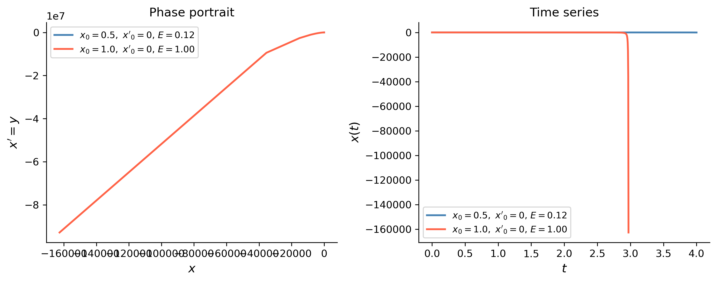
This integral is an elliptic integral — there is no elementary closed form in general, but we can solve the IVP numerically.

Numerical Solution with SciPy

Show the code

def conservative_rhs(t, state):
    x_val, y_val = state
    return [y_val, -3*x_val**2]

t_span = (0, 4)
t_eval = np.linspace(*t_span, 1000)

ics = [(0.5, 0), (1.0, 0)]
colors = ['steelblue', 'tomato']

fig, axes = plt.subplots(1, 2, figsize=(10, 4))

for (x0, y0), color in zip(ics, colors):
    sol = solve_ivp(conservative_rhs, t_span, [x0, y0],
                    t_eval=t_eval, rtol=1e-9, atol=1e-11)
    E = 0.5*y0**2 + x0**3
    label = f'$x_0={x0},\\ x\'_0={y0}$, $E={E:.2f}$'
    axes[0].plot(sol.y[0], sol.y[1], color=color, lw=1.8, label=label)
    axes[1].plot(sol.t, sol.y[0], color=color, lw=1.8, label=label)

axes[0].set_xlabel(r'$x$', fontsize=12)
axes[0].set_ylabel(r"$x' = y$", fontsize=12)
axes[0].set_title('Phase portrait', fontsize=12)
axes[0].legend(fontsize=9)

axes[1].set_xlabel(r'$t$', fontsize=12)
axes[1].set_ylabel(r'$x(t)$', fontsize=12)
axes[1].set_title('Time series', fontsize=12)
axes[1].legend(fontsize=9)

plt.tight_layout()
plt.show()

Figure 3: Phase portrait (left) and time series (right) for the conservative system \(x'' = -3x^2\) with two initial conditions. Trajectories follow curves of constant energy \(E\).

Tip

Pattern. Conservative second-order equation? Form the energy \(E = \tfrac{1}{2}my^2 + V(x)\) and use it as a first integral to reduce the order. When the energy integral cannot be evaluated in elementary form, use scipy.integrate.solve_ivp.

A.11 — Selected Review Exercises with Python

This section works through a few of the longer review exercises from Logan’s Appendix A using Python to check or visualize the answers.

Bifurcation Diagram for \(x' = (x - a)(x^2 - a)\)

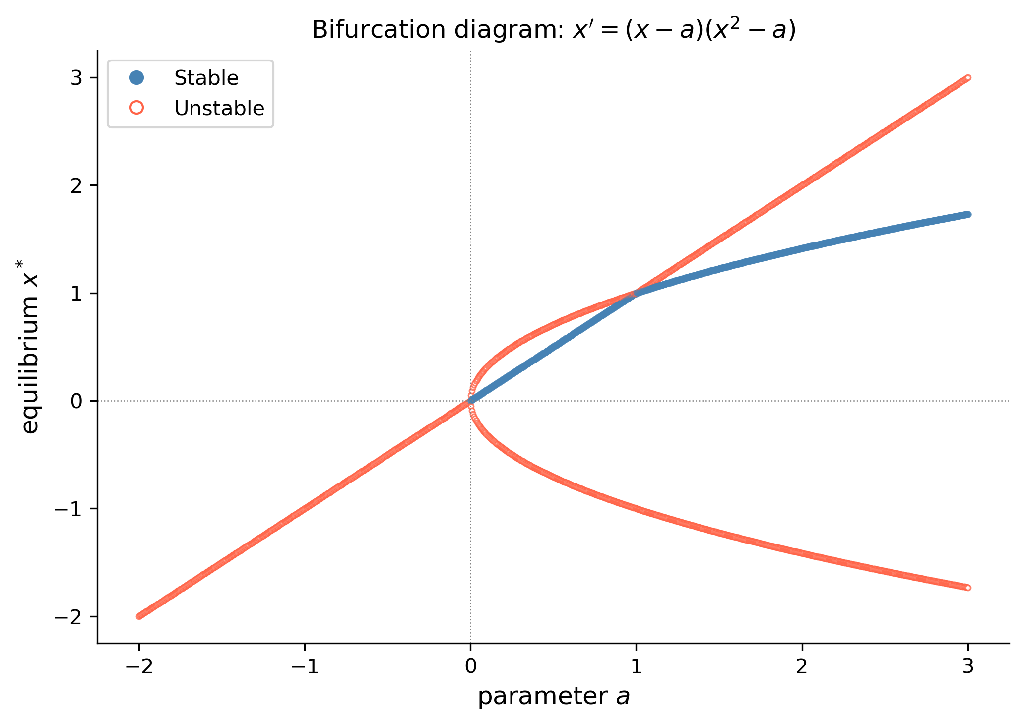
Problem. For all values of the parameter \(a\), find the equilibrium solutions of \(x' = (x-a)(x^2-a)\) and determine their stability. Summarize on a bifurcation diagram (Logan, Review Exercise 4).

Analysis. Setting \(f(x) = (x-a)(x^2-a) = 0\) gives equilibria \(x^* = a\) and \(x^* = \pm\sqrt{a}\) (when \(a \geq 0\)).

For \(a < 0\): only real equilibrium is \(x^* = a\).

For \(a = 0\): triple root at \(x^* = 0\) (degenerate).

For \(a > 0\): three equilibria — \(x^* = -\sqrt{a}\), \(a\), \(\sqrt{a}\) — though \(a\) may coincide with \(\pm\sqrt{a}\) at special values (\(a = 1\): \(x^* = \pm 1\) and \(x^* = 1\), so actually \(x^* = \pm 1\)).

Show the code

a_vals = np.linspace(-2, 3, 800)
fig, ax = plt.subplots(figsize=(7, 5))

for a in a_vals:
    # Equilibria
    equil = [a]
    if a >= 0:
        equil += [np.sqrt(a), -np.sqrt(a)]

    # Stability: sign of f'(x*) = (x^2-a) + (x-a)*2x evaluated at x*
    def f(x):
        return (x - a) * (x**2 - a)
    def df(x):
        return (x**2 - a) + (x - a) * 2*x

    for xstar in equil:
        slope = df(xstar)
        if slope < 0:
            ax.plot(a, xstar, 'o', color='steelblue', ms=2.5, alpha=0.8)
        elif slope > 0:
            ax.plot(a, xstar, 'o', color='tomato',    ms=2.5, alpha=0.8,
                    markerfacecolor='white', markeredgewidth=0.8)
        else:
            ax.plot(a, xstar, 's', color='gray', ms=3, alpha=0.7)

ax.axvline(0, color='gray', lw=0.6, ls=':')
ax.axhline(0, color='gray', lw=0.6, ls=':')
ax.set_xlabel(r'parameter $a$', fontsize=12)
ax.set_ylabel(r'equilibrium $x^*$', fontsize=12)
ax.set_title(r"Bifurcation diagram: $x' = (x-a)(x^2-a)$", fontsize=12)

# Legend proxies
from matplotlib.lines import Line2D
legend_els = [Line2D([0],[0], marker='o', color='steelblue',
                     label='Stable', linestyle='None', ms=6),
              Line2D([0],[0], marker='o', color='tomato', linestyle='None',
                     ms=6, markerfacecolor='white', markeredgewidth=1,
                     label='Unstable')]
ax.legend(handles=legend_els, fontsize=10)
plt.tight_layout()
plt.show()

Figure 4: Bifurcation diagram for \(x' = (x-a)(x^2-a)\). Solid curves: stable equilibria (filled markers); dashed curves: unstable equilibria (open markers).

Evaporating Water Droplet

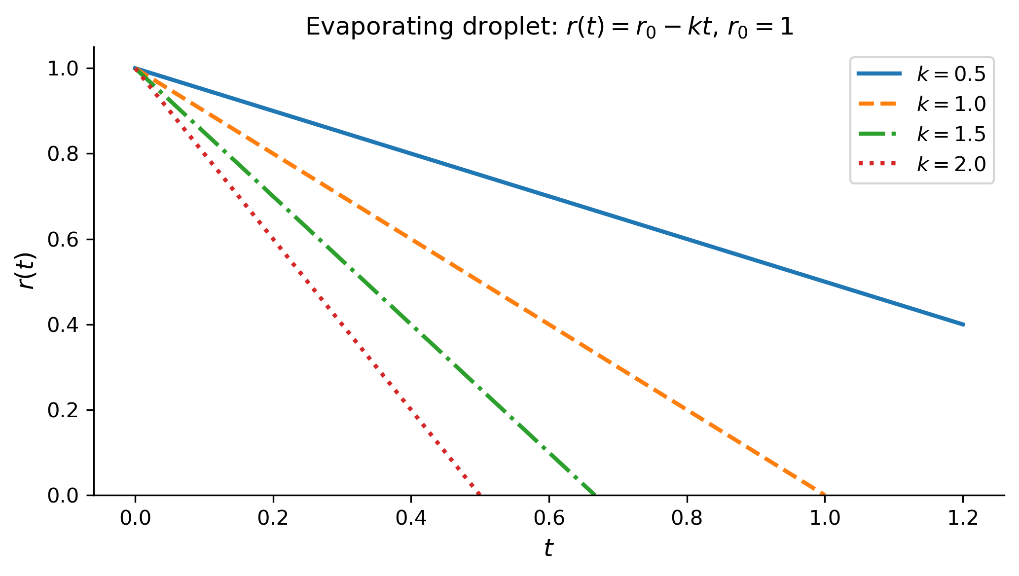
Problem. A spherical droplet loses volume by evaporation at a rate proportional to its surface area. Find \(r = r(t)\) in terms of the proportionality constant \(k > 0\) and initial radius \(r_0\) (Logan, Review Exercise 5).

Solution. Volume \(V = \tfrac{4}{3}\pi r^3\), surface area \(S = 4\pi r^2\).

\[ V' = -k \cdot 4\pi r^2 \quad\Longrightarrow\quad 4\pi r^2 r' = -4k\pi r^2 \quad\Longrightarrow\quad r' = -k. \]

Integrating: \(\boxed{r(t) = r_0 - kt.}\) The droplet vanishes at \(t = r_0/k\).

Show the code

r0 = 1.0
t_max = 1.2

fig, ax = plt.subplots(figsize=(7, 4))

for k, ls in zip([0.5, 1.0, 1.5, 2.0], ['-','--','-.',':']):
    t_end = r0 / k
    t_plot = np.linspace(0, min(t_end, t_max), 300)
    ax.plot(t_plot, np.maximum(r0 - k*t_plot, 0), ls=ls, lw=2,
            label=f'$k={k}$')

ax.set_xlabel(r'$t$', fontsize=12)
ax.set_ylabel(r'$r(t)$', fontsize=12)
ax.set_title(r'Evaporating droplet: $r(t) = r_0 - kt$, $r_0=1$', fontsize=12)
ax.legend(fontsize=10)
ax.set_ylim(bottom=0)
plt.tight_layout()
plt.show()

Figure 5: Radius of an evaporating spherical droplet for several values of the evaporation constant \(k\), with \(r_0 = 1\).

Reduction of Order

Problem. The equation \((1 - t^2)x'' - 2tx' + 2x = 0\) has one solution \(x_1(t) = t\). Find a second linearly independent solution (Logan, Review Exercise 9).

Use reduction of order: set \(x = t\,w(t)\) and substitute.

t = sym.Symbol('t')
x = sym.Function('x')

ode_ro = sym.Eq((1 - t**2)*x(t).diff(t,2) - 2*t*x(t).diff(t) + 2*x(t), 0)

# dsolve finds both solutions
sol_ro = sym.dsolve(ode_ro, x(t))
display(Math(sym.latex(sol_ro)))

\(\displaystyle x{\left(t \right)} = C_{2} \left(- \frac{t^{4}}{3} - t^{2} + 1\right) + C_{1} t + O\left(t^{6}\right)\)

The second solution involves \(\ln\!\left|\tfrac{1+t}{1-t}\right|\), confirming Logan’s result \[ x_2(t) = -1 + \frac{t}{2}\ln\frac{1+t}{1-t}. \]

References

Logan, J David. 2015. A First Course in Differential Equations, Third Edition.

Expand for Session Info

import sys, importlib
print("Python version:", sys.version)
for name in ['numpy', 'sympy', 'scipy', 'matplotlib']:
    mod = importlib.import_module(name)
    print(f"{name}=={mod.__version__}")

Python version: 3.14.4 | packaged by conda-forge | (main, Apr  8 2026, 02:33:53) [Clang 20.1.8 ]
numpy==2.4.3
sympy==1.14.0
scipy==1.17.1
matplotlib==3.10.8

Reuse

CC BY-NC-SA 4.0