Review — Linear and Nonlinear Systems

Show the code

# Imports for the entire session
import numpy as np                          # NumPy for numerical computations
import sympy as sym                         # SymPy for symbolic mathematics
import matplotlib as mpl                    # Matplotlib for plotting
import matplotlib.pyplot as plt             # Matplotlib pyplot interface
from matplotlib.patches import FancyArrowPatch
from scipy.integrate import solve_ivp       # SciPy numerical ODE solver
from IPython.display import Math, display
mpl.rcParams['figure.dpi'] = 150
mpl.rcParams['axes.spines.top'] = False
mpl.rcParams['axes.spines.right'] = False

This document reviews Chapters 4 and 5 of (Logan 2015): Linear Systems (Chapter 4) and Nonlinear Systems (Chapter 5). It is structured as a companion to Review 1 (Chapters 1–2) and Review 2 (Chapter 3): each section states the key idea, works through a representative example by hand, and demonstrates the same calculation or visualization in Python.

The central thread of both chapters is the phase plane: once we write a system of two first-order ODEs as $\mathbf{x}' = \mathbf{f}(\mathbf{x})$, the geometry of solution curves in the $(x_1, x_2)$-plane reveals stability, oscillation, and long-term behavior without solving explicitly.

C.1 — First-Order Systems and the Phase Plane

A first-order system rewrites any $n$th-order ODE — or models any multi-variable process — as \[ \mathbf{x}'(t) = \mathbf{f}(t, \mathbf{x}), \qquad \mathbf{x} = \begin{pmatrix} x_1 \\ x_2 \end{pmatrix},\quad \mathbf{f} = \begin{pmatrix} f_1 \\ f_2 \end{pmatrix}. \]

Converting a second-order ODE to a system (Logan, §4.1). The equation $x'' + bx' + cx = f(t)$ becomes \[ x_1' = x_2, \qquad x_2' = f(t) - bx_2 - cx_1, \] by setting $x_1 = x$ (position) and $x_2 = x'$ (velocity).

By Hand

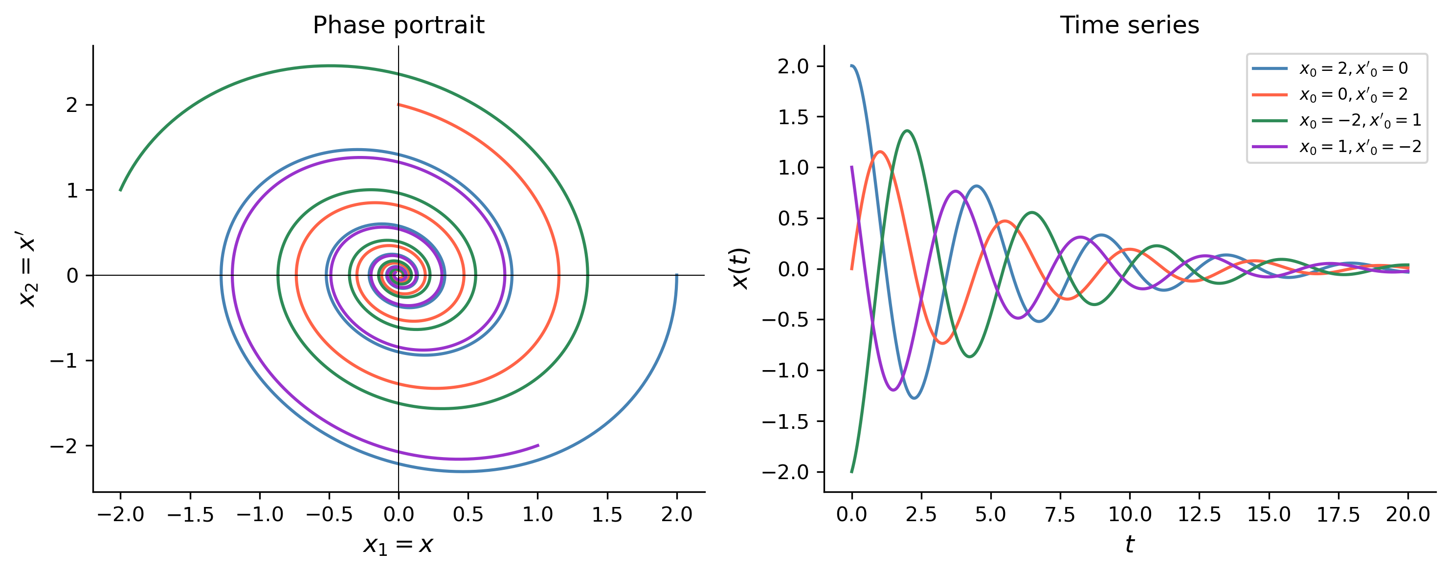
Example. Convert the damped spring–mass equation $x'' + 0.4x' + 2x = 0$ to a first-order system and identify its matrix form.

Let $x_1 = x$, $x_2 = x'$: \[ \begin{pmatrix} x_1' \\ x_2' \end{pmatrix} = \begin{pmatrix} 0 & 1 \\ -2 & -0.4 \end{pmatrix} \begin{pmatrix} x_1 \\ x_2 \end{pmatrix}. \]

Using SymPy

t = sym.Symbol('t')
x = sym.Function('x')

# Original second-order ODE: x'' + 0.4x' + 2x = 0
ode = sym.Eq(x(t).diff(t,2) + sym.Rational(2,5)*x(t).diff(t) + 2*x(t), 0)

# Solve directly to see the solution structure
sol = sym.dsolve(ode, x(t))
display(Math(r'x(t) = ' + sym.latex(sol.rhs)))

# Display the system matrix A
A = sym.Matrix([[0, 1], [-2, sym.Rational(-2,5)]])
display(Math(r'\mathbf{A} = ' + sym.latex(A)))
display(Math(r'\text{eigenvalues: } ' + sym.latex(A.eigenvals())))

$\displaystyle x(t) = \left(C_{1} \sin{\left(\frac{7 t}{5} \right)} + C_{2} \cos{\left(\frac{7 t}{5} \right)}\right) e^{- \frac{t}{5}}$

$\displaystyle \mathbf{A} = \left[\begin{matrix}0 & 1\\-2 & - \frac{2}{5}\end{matrix}\right]$

$\displaystyle \text{eigenvalues: } \left\{ - \frac{1}{5} - \frac{7 i}{5} : 1, \ - \frac{1}{5} + \frac{7 i}{5} : 1\right\}$

Show the code

def damped_osc(t, y):
    return [y[1], -2*y[0] - 0.4*y[1]]

t_span, t_eval = (0, 20), np.linspace(0, 20, 1000)
ics = [(2, 0), (0, 2), (-2, 1), (1, -2)]

fig, axes = plt.subplots(1, 2, figsize=(10, 4))
colors = ['steelblue', 'tomato', 'seagreen', 'darkorchid']

for (x0, v0), color in zip(ics, colors):
    sol = solve_ivp(damped_osc, t_span, [x0, v0],
                    t_eval=t_eval, rtol=1e-9)
    axes[0].plot(sol.y[0], sol.y[1], color=color, lw=1.5)
    axes[1].plot(sol.t,    sol.y[0], color=color, lw=1.5,
                 label=f'$x_0={x0}, x\'_0={v0}$')

axes[0].set_xlabel(r'$x_1 = x$',  fontsize=12)
axes[0].set_ylabel(r"$x_2 = x'$", fontsize=12)
axes[0].set_title('Phase portrait', fontsize=12)
axes[0].axhline(0, color='k', lw=0.5)
axes[0].axvline(0, color='k', lw=0.5)

axes[1].set_xlabel(r'$t$',    fontsize=12)
axes[1].set_ylabel(r'$x(t)$', fontsize=12)
axes[1].set_title('Time series', fontsize=12)
axes[1].legend(fontsize=8)

plt.tight_layout()
plt.show()

Figure 1: Phase portrait (left) and time series (right) for the damped oscillator $x''+0.4x'+2x=0$. All trajectories spiral into the origin (stable spiral).

Tip

Pattern. To convert an $n$th-order ODE to a system: let $x_1 = x,\; x_2 = x',\;\ldots,\; x_n = x^{(n-1)}$. The resulting system matrix $\mathbf{A}$ is called the companion matrix of the ODE.

C.2 — Matrix Algebra Essentials

A linear system $\mathbf{x}' = A\mathbf{x}$ (constant $2\times 2$ matrix $A$) governs the dynamics near equilibria. Key definitions (Logan, §4.2):

Determinant: $\det A = ad - bc$ for $A = \bigl(\begin{smallmatrix}a&b\\c&d\end{smallmatrix}\bigr)$.
Trace: $\text{tr}\,A = a + d$.
Characteristic equation: $\det(A - \lambda I) = 0$, i.e.
$\lambda^2 - (\text{tr}\,A)\lambda + \det A = 0$.
Eigenvector: $A\mathbf{v} = \lambda\mathbf{v}$, $\mathbf{v} \neq \mathbf{0}$.

An equilibrium of $\mathbf{x}' = A\mathbf{x}$ is at the origin.

By Hand

Example. Find the eigenvalues and eigenvectors of $A = \begin{pmatrix} 1 & 2 \\ 3 & 2 \end{pmatrix}$ (Logan, §4.3).

Characteristic equation: $\lambda^2 - 3\lambda + (2 - 6) = \lambda^2 - 3\lambda - 4 = (\lambda-4)(\lambda+1) = 0$.

Eigenvalues: $\lambda_1 = 4$, $\lambda_2 = -1$.

Eigenvector for $\lambda_1 = 4$: $(A - 4I)\mathbf{v} = \mathbf{0}$: $\begin{pmatrix}-3&2\\3&-2\end{pmatrix}\mathbf{v} = \mathbf{0}$ $\Rightarrow \mathbf{v}_1 = \begin{pmatrix}2\\3\end{pmatrix}$.

Eigenvector for $\lambda_2 = -1$: $\begin{pmatrix}2&2\\3&3\end{pmatrix}\mathbf{v} = \mathbf{0}$ $\Rightarrow \mathbf{v}_2 = \begin{pmatrix}1\\-1\end{pmatrix}$.

Using SymPy

A_ex = sym.Matrix([[1, 2], [3, 2]])

evals = A_ex.eigenvals()
evecs = A_ex.eigenvects()

display(Math(r'A = ' + sym.latex(A_ex)))
display(Math(r'\det A = ' + sym.latex(A_ex.det())
             + r',\quad \mathrm{tr}\,A = ' + sym.latex(A_ex.trace())))
display(Math(r'\text{Characteristic polynomial: }'
             + sym.latex(sym.factor(A_ex.charpoly().as_expr()))))

for lam, mult, vecs in evecs:
    display(Math(r'\lambda = ' + sym.latex(lam)
                 + r',\quad \mathbf{v} = ' + sym.latex(vecs[0])))

$\displaystyle A = \left[\begin{matrix}1 & 2\\3 & 2\end{matrix}\right]$

$\displaystyle \det A = -4,\quad \mathrm{tr}\,A = 3$

$\displaystyle \text{Characteristic polynomial: }\left(\lambda - 4\right) \left(\lambda + 1\right)$

$\displaystyle \lambda = -1,\quad \mathbf{v} = \left[\begin{matrix}-1\\1\end{matrix}\right]$

$\displaystyle \lambda = 4,\quad \mathbf{v} = \left[\begin{matrix}\frac{2}{3}\\1\end{matrix}\right]$

Tip

Pattern. For $2\times 2$ systems, the characteristic equation $\lambda^2 - (\text{tr}\,A)\lambda + \det A = 0$ gives eigenvalues from trace and determinant alone — no row reduction needed.

C.3 — Solving Linear Systems: Real Unequal Eigenvalues

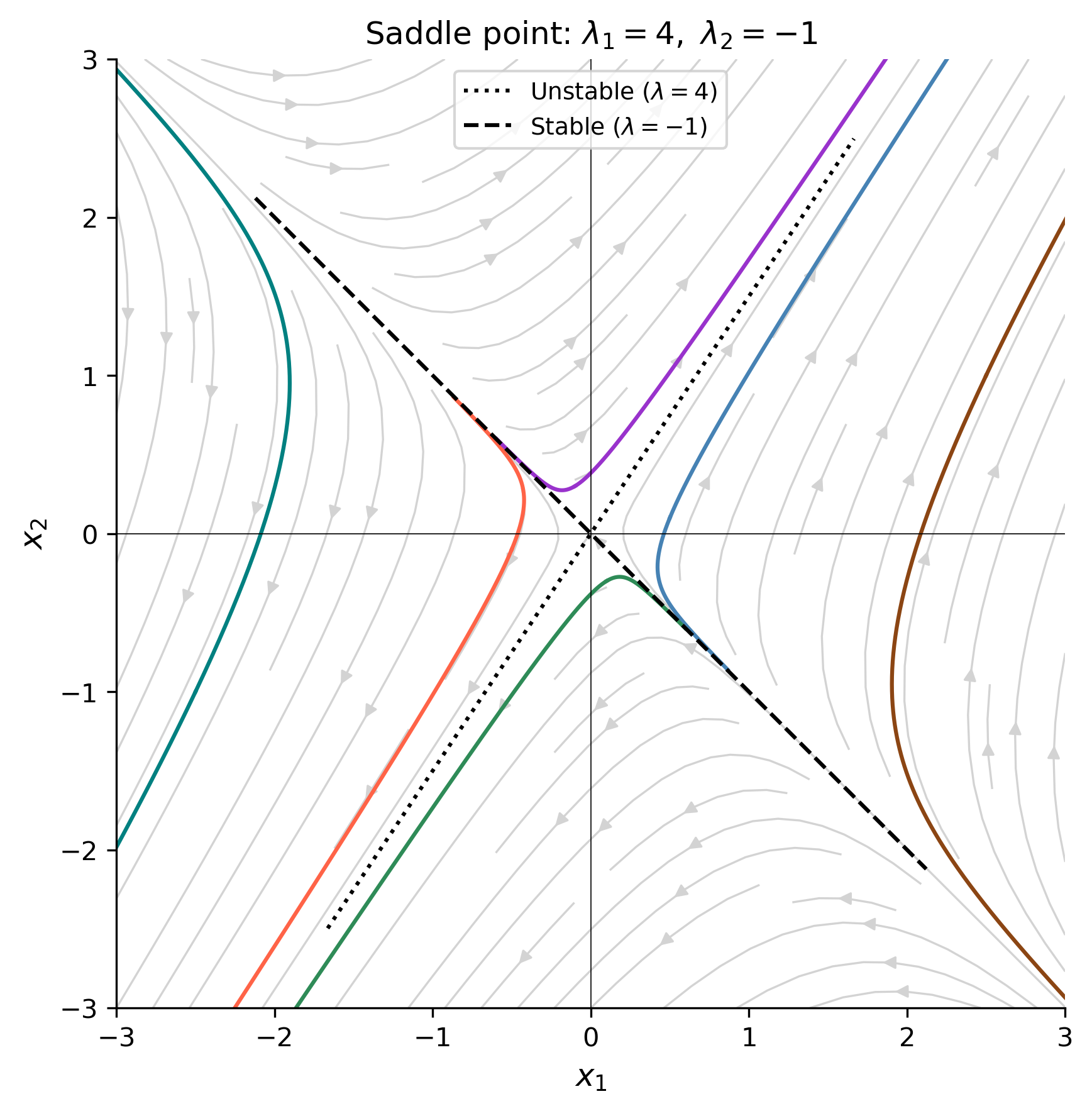
When $A$ has two real, distinct eigenvalues $\lambda_1 \neq \lambda_2$ with eigenvectors $\mathbf{v}_1$, $\mathbf{v}_2$, the general solution is (Logan, §4.4.1) \[ \mathbf{x}(t) = c_1\,e^{\lambda_1 t}\mathbf{v}_1 + c_2\,e^{\lambda_2 t}\mathbf{v}_2. \]

Equilibrium classification from the sign of the eigenvalues:

Signs of $\lambda_1, \lambda_2$	Equilibrium type
Both negative	Stable node (sink)
Both positive	Unstable node (source)
Opposite signs	Saddle point

By Hand

Example. Solve $\mathbf{x}' = \begin{pmatrix}1&2\\3&2\end{pmatrix}\mathbf{x}$ with $\mathbf{x}(0) = \begin{pmatrix}1\\0\end{pmatrix}$ (Logan, §4.4.1).

Eigenvalues $\lambda_1 = 4$, $\lambda_2 = -1$ (opposite signs → saddle).

General solution: \[ \mathbf{x}(t) = c_1 e^{4t}\begin{pmatrix}2\\3\end{pmatrix} + c_2 e^{-t}\begin{pmatrix}1\\-1\end{pmatrix}. \]

Apply $\mathbf{x}(0) = (1,0)^T$: $2c_1 + c_2 = 1$, $3c_1 - c_2 = 0$. Solving: $c_1 = 1/5$, $c_2 = 3/5$.

\[ \mathbf{x}(t) = \frac{1}{5}e^{4t}\begin{pmatrix}2\\3\end{pmatrix} + \frac{3}{5}e^{-t}\begin{pmatrix}1\\-1\end{pmatrix}. \]

Using SymPy and Matplotlib

t  = sym.Symbol('t')
A1 = sym.Matrix([[1, 2], [3, 2]])
x0 = sym.Matrix([1, 0])

# General solution via matrix exponential
sol_sys = sym.dsolve(
    [sym.Eq(sym.Function('x1')(t).diff(t), A1[0,0]*sym.Function('x1')(t)
                                            + A1[0,1]*sym.Function('x2')(t)),
     sym.Eq(sym.Function('x2')(t).diff(t), A1[1,0]*sym.Function('x1')(t)
                                            + A1[1,1]*sym.Function('x2')(t))],
)
for eq in sol_sys:
    display(Math(sym.latex(eq)))

$\displaystyle x_{1}{\left(t \right)} = - C_{1} e^{- t} + \frac{2 C_{2} e^{4 t}}{3}$

$\displaystyle x_{2}{\left(t \right)} = C_{1} e^{- t} + C_{2} e^{4 t}$

Show the code

def saddle_rhs(t, y):
    return [y[0] + 2*y[1], 3*y[0] + 2*y[1]]

fig, ax = plt.subplots(figsize=(6, 6))

# Stream plot background
x1g = np.linspace(-3, 3, 22)
x2g = np.linspace(-3, 3, 22)
X1, X2 = np.meshgrid(x1g, x2g)
dX1 = X1 + 2*X2
dX2 = 3*X1 + 2*X2
speed = np.sqrt(dX1**2 + dX2**2)
speed[speed == 0] = 1
ax.streamplot(X1, X2, dX1/speed, dX2/speed,
              density=0.9, color='lightgray', linewidth=0.8)

# Sample trajectories
colors = ['steelblue', 'tomato', 'seagreen', 'darkorchid',
          'saddlebrown', 'teal']
ics_saddle = [(0.5, 0.1), (-0.5, -0.1), (0.1, -0.3),
              (-0.1, 0.3), (2.5, 1.0), (-2.5, -1.0)]
def escaped(y, limit=4.0):
    """Return index of first point outside the plot box, or len."""
    outside = np.where(np.max(np.abs(y), axis=0) > limit)[0]
    return outside[0] if len(outside) else y.shape[1]

for (x10, x20), color in zip(ics_saddle, colors):
    for t_sp in [(0, 1.2), (0, -1.2)]:
        sol = solve_ivp(saddle_rhs, t_sp, [x10, x20],
                        t_eval=np.linspace(*t_sp, 300), rtol=1e-9)
        idx = escaped(sol.y)
        ax.plot(sol.y[0, :idx], sol.y[1, :idx], color=color, lw=1.5)

# Eigenvectors
v1 = np.array([2, 3]) / np.linalg.norm([2, 3])
v2 = np.array([1, -1]) / np.linalg.norm([1, -1])
for v, ls, lbl in [(v1, ':', 'Unstable ($\\lambda=4$)'),
                   (v2, '--', 'Stable ($\\lambda=-1$)')]:
    ax.plot([-3*v[0], 3*v[0]], [-3*v[1], 3*v[1]],
            ls=ls, color='k', lw=1.5, label=lbl)

ax.set_xlim(-3, 3); ax.set_ylim(-3, 3)
ax.set_xlabel(r'$x_1$', fontsize=12)
ax.set_ylabel(r'$x_2$', fontsize=12)
ax.set_title('Saddle point: $\\lambda_1=4,\\ \\lambda_2=-1$', fontsize=12)
ax.legend(fontsize=9); ax.set_aspect('equal')
ax.axhline(0, color='k', lw=0.4); ax.axvline(0, color='k', lw=0.4)
plt.tight_layout()
plt.show()

Figure 2: Phase portrait for $\mathbf{x}' = A\mathbf{x}$ with eigenvalues $\lambda_1=4$ (unstable) and $\lambda_2=-1$ (stable). The origin is a **saddle point**: trajectories approach along the stable manifold (dashed) and are repelled along the unstable manifold (dotted).

C.4 — Complex Eigenvalues: Spirals and Centers

When $A$ has complex eigenvalues $\lambda = \alpha \pm \beta i$ ($\beta \neq 0$), Euler’s formula gives two real solutions (Logan, §4.4.2): \[ \mathbf{x}_1(t) = e^{\alpha t}(\mathbf{a}\cos\beta t - \mathbf{b}\sin\beta t), \quad \mathbf{x}_2(t) = e^{\alpha t}(\mathbf{a}\sin\beta t + \mathbf{b}\cos\beta t), \] where $\mathbf{v} = \mathbf{a} + i\mathbf{b}$ is a complex eigenvector.

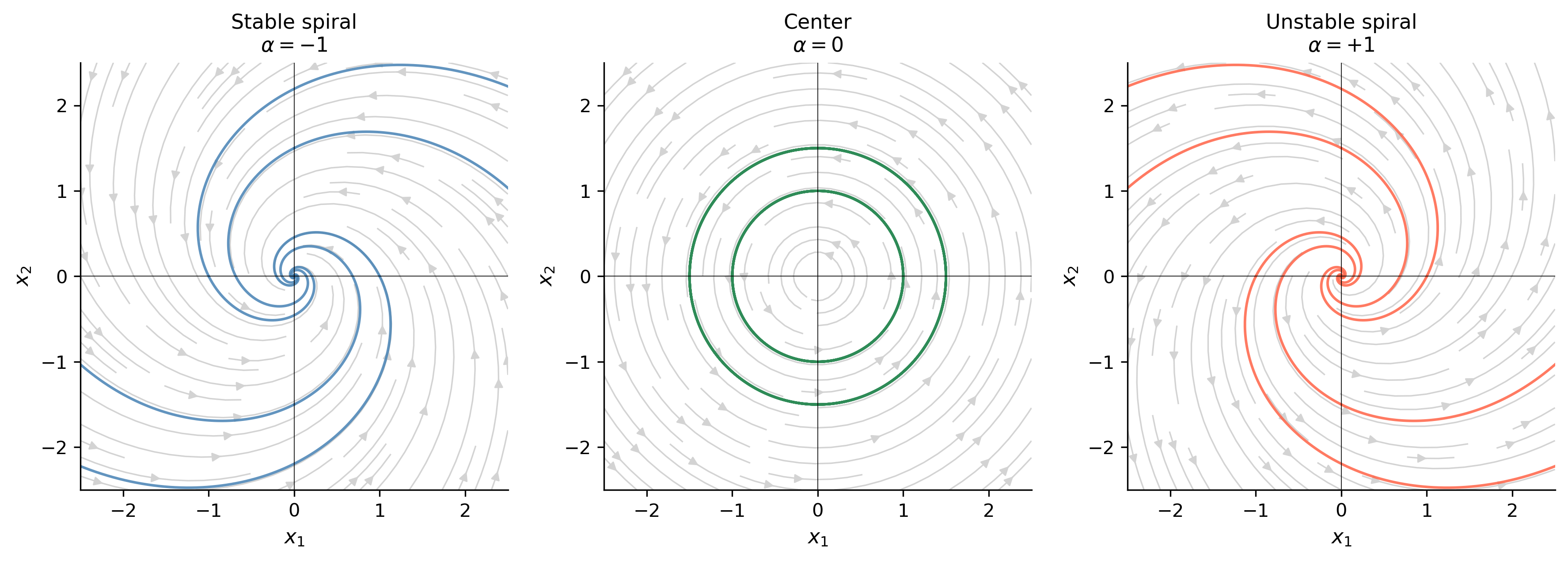
Classification by $\alpha = \text{Re}(\lambda)$:

$\alpha$	Equilibrium type
$\alpha < 0$	Stable spiral (sink)
$\alpha > 0$	Unstable spiral (source)
$\alpha = 0$	Center (neutrally stable)

By Hand

Example. Solve $\mathbf{x}' = \begin{pmatrix}-1&-2\\2&-1\end{pmatrix}\mathbf{x}$ (Logan, §4.4.2).

Characteristic equation: $\lambda^2 + 2\lambda + 5 = 0$, roots $\lambda = -1 \pm 2i$.

Eigenvector for $\lambda = -1 + 2i$: $(A - (-1+2i)I)\mathbf{v} = \mathbf{0}$: $\begin{pmatrix}-2i&-2\\2&-2i\end{pmatrix}\mathbf{v} = \mathbf{0}$ $\Rightarrow \mathbf{v} = \begin{pmatrix}1\\-i\end{pmatrix} = \begin{pmatrix}1\\0\end{pmatrix} + i\begin{pmatrix}0\\-1\end{pmatrix}$.

So $\mathbf{a} = (1,0)^T$, $\mathbf{b} = (0,-1)^T$, $\alpha = -1$, $\beta = 2$.

\[ \boxed{\mathbf{x}(t) = c_1 e^{-t}\begin{pmatrix}\cos 2t\\\sin 2t\end{pmatrix} + c_2 e^{-t}\begin{pmatrix}-\sin 2t\\\cos 2t\end{pmatrix}.} \]

This is a stable spiral: oscillations that decay as $t\to\infty$.

Using SymPy and Matplotlib

t = sym.Symbol('t')
A2 = sym.Matrix([[-1, -2], [2, -1]])

display(Math(r'A = ' + sym.latex(A2)))
display(Math(r'\text{eigenvalues: } ' + sym.latex(list(A2.eigenvals().keys()))))

x1f, x2f = sym.Function('x1'), sym.Function('x2')
sys2 = [sym.Eq(x1f(t).diff(t), -x1f(t) - 2*x2f(t)),
        sym.Eq(x2f(t).diff(t),  2*x1f(t) - x2f(t))]
sol2 = sym.dsolve(sys2)
for eq in sol2:
    display(Math(sym.latex(eq)))

$\displaystyle A = \left[\begin{matrix}-1 & -2\\2 & -1\end{matrix}\right]$

$\displaystyle \text{eigenvalues: } \left[ -1 - 2 i, \ -1 + 2 i\right]$

$\displaystyle x_{1}{\left(t \right)} = - C_{1} e^{- t} \sin{\left(2 t \right)} - C_{2} e^{- t} \cos{\left(2 t \right)}$

$\displaystyle x_{2}{\left(t \right)} = C_{1} e^{- t} \cos{\left(2 t \right)} - C_{2} e^{- t} \sin{\left(2 t \right)}$

Show the code

systems = [
    (lambda t, y: [-y[0]-2*y[1],  2*y[0]-y[1]],  'Stable spiral\n$\\alpha=-1$',    'steelblue'),
    (lambda t, y: [        -2*y[1],  2*y[0]      ],  'Center\n$\\alpha=0$',          'seagreen'),
    (lambda t, y: [ y[0]-2*y[1],   2*y[0]+y[1]  ],  'Unstable spiral\n$\\alpha=+1$', 'tomato'),
]

fig, axes = plt.subplots(1, 3, figsize=(12, 4))
ics_c = [(1, 0), (-1, 0), (0, 1.5), (0, -1.5)]

for ax, (rhs, title, color) in zip(axes, systems):
    x1g = np.linspace(-2.5, 2.5, 20)
    X1c, X2c = np.meshgrid(x1g, x1g)
    dX1c = np.array([[rhs(0,[xi,yi])[0] for xi in x1g] for yi in x1g])
    dX2c = np.array([[rhs(0,[xi,yi])[1] for xi in x1g] for yi in x1g])
    spd  = np.sqrt(dX1c**2 + dX2c**2); spd[spd==0] = 1
    ax.streamplot(X1c, X2c, dX1c/spd, dX2c/spd,
                  density=0.9, color='lightgray', linewidth=0.8)

    t_fwd = np.linspace(0,  6, 600)
    t_bwd = np.linspace(0, -6, 600)
    for ic in ics_c:
        for t_ev in [t_fwd, t_bwd]:
            s = solve_ivp(rhs, (t_ev[0], t_ev[-1]), list(ic),
                          t_eval=t_ev, rtol=1e-9)
            idx = escaped(s.y, limit=3.0)
            ax.plot(s.y[0, :idx], s.y[1, :idx],
                    color=color, lw=1.4, alpha=0.85)

    ax.set_xlim(-2.5, 2.5); ax.set_ylim(-2.5, 2.5)
    ax.axhline(0, color='k', lw=0.4); ax.axvline(0, color='k', lw=0.4)
    ax.set_xlabel(r'$x_1$', fontsize=11)
    ax.set_ylabel(r'$x_2$', fontsize=11)
    ax.set_title(title, fontsize=11)
    ax.set_aspect('equal')

plt.tight_layout()
plt.show()

Figure 3: Phase portraits for three qualitative types arising from complex eigenvalues $\lambda = \alpha \pm \beta i$. Left: stable spiral ($\alpha<0$). Center: center ($\alpha=0$). Right: unstable spiral ($\alpha>0$).

Tip

Pattern. Complex eigenvalues $\alpha \pm \beta i$: the real part $\alpha$ controls whether trajectories spiral in ($\alpha<0$), spiral out ($\alpha>0$), or orbit ($\alpha=0$); the imaginary part $\beta$ sets the angular frequency.

C.5 — Repeated Eigenvalues

When $A$ has a repeated eigenvalue $\lambda$ (Logan, §4.4.3), two cases arise.

Case 1 — Two independent eigenvectors (rare for $2\times2$): the general solution is $\mathbf{x}=e^{\lambda t}(c_1\mathbf{v}_1 + c_2\mathbf{v}_2)$ (star node).

Case 2 — One eigenvector (typical): find a generalized eigenvector $\mathbf{w}$ satisfying $(A-\lambda I)\mathbf{w} = \mathbf{v}$. Then \[ \mathbf{x}(t) = c_1 e^{\lambda t}\mathbf{v} + c_2 e^{\lambda t}(t\mathbf{v} + \mathbf{w}). \]

By Hand

Example. Solve $\mathbf{x}' = \begin{pmatrix}3&1\\0&3\end{pmatrix}\mathbf{x}$ (Logan, §4.4.3).

Characteristic equation: $(\lambda-3)^2 = 0 \Rightarrow \lambda = 3$ (repeated).

Eigenvector: $(A - 3I)\mathbf{v} = \begin{pmatrix}0&1\\0&0\end{pmatrix}\mathbf{v}=\mathbf{0}$ $\Rightarrow \mathbf{v} = \begin{pmatrix}1\\0\end{pmatrix}$.

Generalized eigenvector: $(A-3I)\mathbf{w} = \mathbf{v}$: $\begin{pmatrix}0&1\\0&0\end{pmatrix}\mathbf{w} = \begin{pmatrix}1\\0\end{pmatrix}$ $\Rightarrow \mathbf{w} = \begin{pmatrix}0\\1\end{pmatrix}$.

General solution: \[ \boxed{\mathbf{x}(t) = c_1 e^{3t}\begin{pmatrix}1\\0\end{pmatrix} + c_2 e^{3t}\!\left(t\begin{pmatrix}1\\0\end{pmatrix} + \begin{pmatrix}0\\1\end{pmatrix}\right).} \]

t = sym.Symbol('t')
A3 = sym.Matrix([[3, 1], [0, 3]])

display(Math(r'A = ' + sym.latex(A3)))
display(Math(r'\text{eigenvalues: } ' + sym.latex(list(A3.eigenvals().keys()))))

x1f, x2f = sym.Function('x1'), sym.Function('x2')
sys3 = [sym.Eq(x1f(t).diff(t), 3*x1f(t) + x2f(t)),
        sym.Eq(x2f(t).diff(t), 3*x2f(t))]
sol3 = sym.dsolve(sys3)
for eq in sol3:
    display(Math(sym.latex(eq)))

$\displaystyle A = \left[\begin{matrix}3 & 1\\0 & 3\end{matrix}\right]$

$\displaystyle \text{eigenvalues: } \left[ 3\right]$

$\displaystyle x_{1}{\left(t \right)} = C_{1} e^{3 t} + C_{2} t e^{3 t}$

$\displaystyle x_{2}{\left(t \right)} = C_{2} e^{3 t}$

C.6 — Phase Plane Analysis and Equilibrium Classification

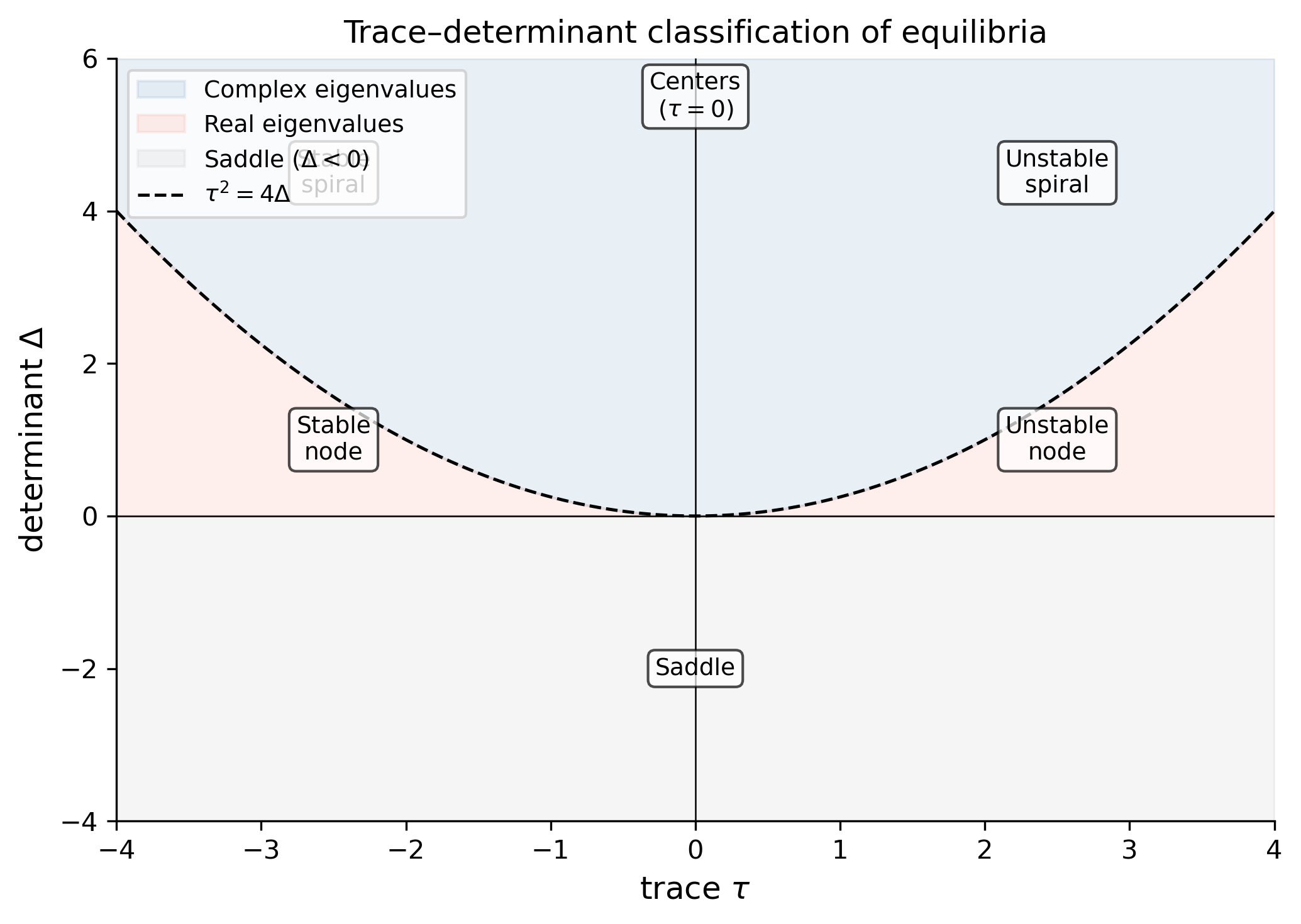
For a $2\times2$ linear system $\mathbf{x}' = A\mathbf{x}$, the complete classification of the equilibrium at the origin depends on the trace $\tau = \text{tr}\,A$ and determinant $\Delta = \det A$ (Logan, §4.5):

\[ \lambda_{1,2} = \frac{\tau \pm \sqrt{\tau^2 - 4\Delta}}{2}. \]

Region in $(\Delta, \tau)$-plane	Equilibrium type
$\Delta < 0$	Saddle
$\Delta > 0$, $\tau^2 - 4\Delta > 0$, $\tau < 0$	Stable node
$\Delta > 0$, $\tau^2 - 4\Delta > 0$, $\tau > 0$	Unstable node
$\Delta > 0$, $\tau^2 - 4\Delta < 0$, $\tau < 0$	Stable spiral
$\Delta > 0$, $\tau^2 - 4\Delta < 0$, $\tau > 0$	Unstable spiral
$\Delta > 0$, $\tau = 0$	Center

Classification Diagram

Show the code

fig, ax = plt.subplots(figsize=(7, 5))

tau_arr = np.linspace(-4, 4, 400)

# Parabola tau^2 = 4*Delta
ax.fill_between(tau_arr, tau_arr**2/4, 6,
                alpha=0.12, color='steelblue', label='Complex eigenvalues')
ax.fill_between(tau_arr, 0, tau_arr**2/4,
                alpha=0.10, color='tomato',    label='Real eigenvalues')
ax.fill_between(tau_arr, -4, 0,
                alpha=0.08, color='gray',      label='Saddle ($\\Delta<0$)')
ax.plot(tau_arr, tau_arr**2/4, 'k--', lw=1.2, label=r'$\tau^2 = 4\Delta$')
ax.axhline(0, color='k', lw=0.6)
ax.axvline(0, color='k', lw=0.6)

labels = {
    (-2.5, 4.5): 'Stable\nspiral',
    ( 2.5, 4.5): 'Unstable\nspiral',
    ( 0.0, 5.5): 'Centers\n($\\tau=0$)',
    (-2.5, 1.0): 'Stable\nnode',
    ( 2.5, 1.0): 'Unstable\nnode',
    ( 0.0,-2.0): 'Saddle',
}
for (tx, ty), txt in labels.items():
    ax.text(tx, ty, txt, ha='center', va='center', fontsize=9,
            bbox=dict(boxstyle='round,pad=0.3', fc='white', alpha=0.7))

ax.set_xlim(-4, 4); ax.set_ylim(-4, 6)
ax.set_xlabel(r'trace $\tau$', fontsize=12)
ax.set_ylabel(r'determinant $\Delta$', fontsize=12)
ax.set_title('Trace–determinant classification of equilibria', fontsize=12)
ax.legend(fontsize=9, loc='upper left')
plt.tight_layout()
plt.show()

Figure 4: The trace–determinant plane classifying equilibria of $\mathbf{x}'=A\mathbf{x}$. The parabola $\tau^2 = 4\Delta$ separates real (outside) from complex (inside) eigenvalues. The vertical axis $\tau=0$ separates stable (left) from unstable (right).

# Quick Python classifier: given A, report the equilibrium type
def classify_equilibrium(A_mat):
    tr  = float(A_mat.trace())
    det = float(A_mat.det())
    disc = tr**2 - 4*det
    if det < 0:
        return "Saddle"
    elif disc > 0:
        return "Stable node" if tr < 0 else "Unstable node"
    elif disc < 0:
        return "Stable spiral" if tr < 0 else (
               "Unstable spiral" if tr > 0 else "Center")
    else:
        return "Star node / degenerate"

examples = [
    sym.Matrix([[1,  2], [3,  2]]),   # saddle
    sym.Matrix([[-1,-2], [2, -1]]),   # stable spiral
    sym.Matrix([[ 1, 2], [-2, 1]]),   # unstable spiral
    sym.Matrix([[ 0,-2], [2,  0]]),   # center
    sym.Matrix([[-2, 0], [0, -3]]),   # stable node
]
for M in examples:
    etype = classify_equilibrium(M)
    evals_str = [str(sym.simplify(e)) for e in M.eigenvals()]
    print(f"A = {list(M.tolist())}  →  {etype}   (eigenvalues: {evals_str})")

A = [[1, 2], [3, 2]]  →  Saddle   (eigenvalues: ['4', '-1'])
A = [[-1, -2], [2, -1]]  →  Stable spiral   (eigenvalues: ['-1 - 2*I', '-1 + 2*I'])
A = [[1, 2], [-2, 1]]  →  Unstable spiral   (eigenvalues: ['1 - 2*I', '1 + 2*I'])
A = [[0, -2], [2, 0]]  →  Center   (eigenvalues: ['-2*I', '2*I'])
A = [[-2, 0], [0, -3]]  →  Stable node   (eigenvalues: ['-2', '-3'])

C.7 — Nonhomogeneous Linear Systems

The system $\mathbf{x}' = A\mathbf{x} + \mathbf{f}(t)$ with a forcing term $\mathbf{f}(t)$ has general solution (Logan, §4.6) \[ \mathbf{x}(t) = \mathbf{x}_h(t) + \mathbf{x}_p(t), \] where $\mathbf{x}_h$ solves the homogeneous system and $\mathbf{x}_p$ is any particular solution. The variation of parameters formula gives \[ \mathbf{x}_p(t) = \Phi(t)\int \Phi(t)^{-1}\mathbf{f}(t)\,dt, \] where $\Phi(t)$ is the fundamental matrix whose columns are the two independent solutions.

By Hand

Example. Solve $\mathbf{x}' = \begin{pmatrix}0&1\\-1&0\end{pmatrix}\mathbf{x} + \begin{pmatrix}0\\1\end{pmatrix}$ (a forced harmonic oscillator).

Homogeneous: $\lambda = \pm i$ (center), so $\mathbf{x}_h = c_1\begin{pmatrix}\cos t\\\!-\!\sin t\end{pmatrix} + c_2\begin{pmatrix}\sin t\\\cos t\end{pmatrix}$.

For the particular solution, try $\mathbf{x}_p = \begin{pmatrix}a\\b\end{pmatrix}$ (constant). Substituting: $\begin{pmatrix}0\\0\end{pmatrix} = \begin{pmatrix}b\\-a+1\end{pmatrix}$, giving $b = 0$, $a = 1$.

\[ \mathbf{x}(t) = c_1\begin{pmatrix}\cos t\\-\sin t\end{pmatrix} + c_2\begin{pmatrix}\sin t\\\cos t\end{pmatrix} + \begin{pmatrix}1\\0\end{pmatrix}. \]

t = sym.Symbol('t')
x1f, x2f = sym.Function('x1'), sym.Function('x2')

sys_nh = [sym.Eq(x1f(t).diff(t),  x2f(t)),
          sym.Eq(x2f(t).diff(t), -x1f(t) + 1)]
sol_nh = sym.dsolve(sys_nh)
for eq in sol_nh:
    display(Math(sym.latex(sym.simplify(eq))))

$\displaystyle x_{1}{\left(t \right)} = C_{1} \sin{\left(t \right)} + C_{2} \cos{\left(t \right)} + 1$

$\displaystyle x_{2}{\left(t \right)} = C_{1} \cos{\left(t \right)} - C_{2} \sin{\left(t \right)}$

C.8 — Linearization of Nonlinear Systems

For a nonlinear autonomous system $\mathbf{x}' = \mathbf{f}(\mathbf{x})$, let $\mathbf{x}^*$ be an equilibrium ($\mathbf{f}(\mathbf{x}^*) = \mathbf{0}$). The Jacobian matrix at $\mathbf{x}^*$ is (Logan, §5.1) \[ J(\mathbf{x}^*) = \begin{pmatrix} \partial f_1/\partial x_1 & \partial f_1/\partial x_2 \\ \partial f_2/\partial x_1 & \partial f_2/\partial x_2 \end{pmatrix}_{\mathbf{x}=\mathbf{x}^*}. \] The linearized system $\mathbf{u}' = J(\mathbf{x}^*)\mathbf{u}$ (where $\mathbf{u} = \mathbf{x} - \mathbf{x}^*$) approximates the nonlinear dynamics near the equilibrium, and its eigenvalues determine local stability — provided neither eigenvalue has zero real part (hyperbolic equilibrium).

By Hand

Example. Find and classify the equilibria of the nonlinear system (Logan, §5.1) \[ x_1' = x_1 - x_1 x_2, \qquad x_2' = -x_2 + x_1 x_2. \] (This is the Lotka–Volterra predator–prey model with $r = K = 1$.)

Equilibria. Set $f_1 = f_2 = 0$: $x_1(1 - x_2) = 0$ and $x_2(-1 + x_1) = 0$. Solutions: $(0, 0)$ and $(1, 1)$.

Jacobian. \[ J = \begin{pmatrix}1 - x_2 & -x_1 \\ x_2 & x_1 - 1\end{pmatrix}. \]

At $(0,0)$: $J = \begin{pmatrix}1&0\\0&-1\end{pmatrix}$, eigenvalues $\lambda = 1, -1$ → saddle (unstable).

At $(1,1)$: $J = \begin{pmatrix}0&-1\\1&0\end{pmatrix}$, eigenvalues $\lambda = \pm i$ → center (neutrally stable in the linearization; nonlinear analysis confirms it is a true center for this model).

Using SymPy

x1, x2 = sym.symbols('x1 x2')

# Lotka-Volterra system
f1 =  x1 - x1*x2
f2 = -x2 + x1*x2

F = sym.Matrix([f1, f2])
X = sym.Matrix([x1, x2])
J = F.jacobian(X)
display(Math(r'J(\mathbf{x}) = ' + sym.latex(J)))

# Find equilibria
equil = sym.solve([f1, f2], [x1, x2])
print("Equilibria:", equil)

# Classify each
for eq in equil:
    J_eq = J.subs([(x1, eq[0]), (x2, eq[1])])
    evals = list(J_eq.eigenvals().keys())
    etype = classify_equilibrium(J_eq)
    display(Math(r'\mathbf{x}^* = ' + sym.latex(sym.Matrix(list(eq)))
                 + r',\quad J = ' + sym.latex(J_eq)
                 + r',\quad \lambda = ' + sym.latex(evals)
                 + r'\quad\Rightarrow\quad\text{' + etype + '}'))

$\displaystyle J(\mathbf{x}) = \left[\begin{matrix}1 - x_{2} & - x_{1}\\x_{2} & x_{1} - 1\end{matrix}\right]$

Equilibria: [(0, 0), (1, 1)]

$\displaystyle \mathbf{x}^* = \left[\begin{matrix}0\\0\end{matrix}\right],\quad J = \left[\begin{matrix}1 & 0\\0 & -1\end{matrix}\right],\quad \lambda = \left[ 1, \ -1\right]\quad\Rightarrow\quad\text{Saddle}$

$\displaystyle \mathbf{x}^* = \left[\begin{matrix}1\\1\end{matrix}\right],\quad J = \left[\begin{matrix}0 & -1\\1 & 0\end{matrix}\right],\quad \lambda = \left[ - i, \ i\right]\quad\Rightarrow\quad\text{Center}$

Tip

Pattern. For a nonlinear system: (1) find equilibria by setting $\mathbf{f} = \mathbf{0}$; (2) compute $J$ symbolically; (3) evaluate $J$ at each equilibrium and classify using trace/determinant or eigenvalues.

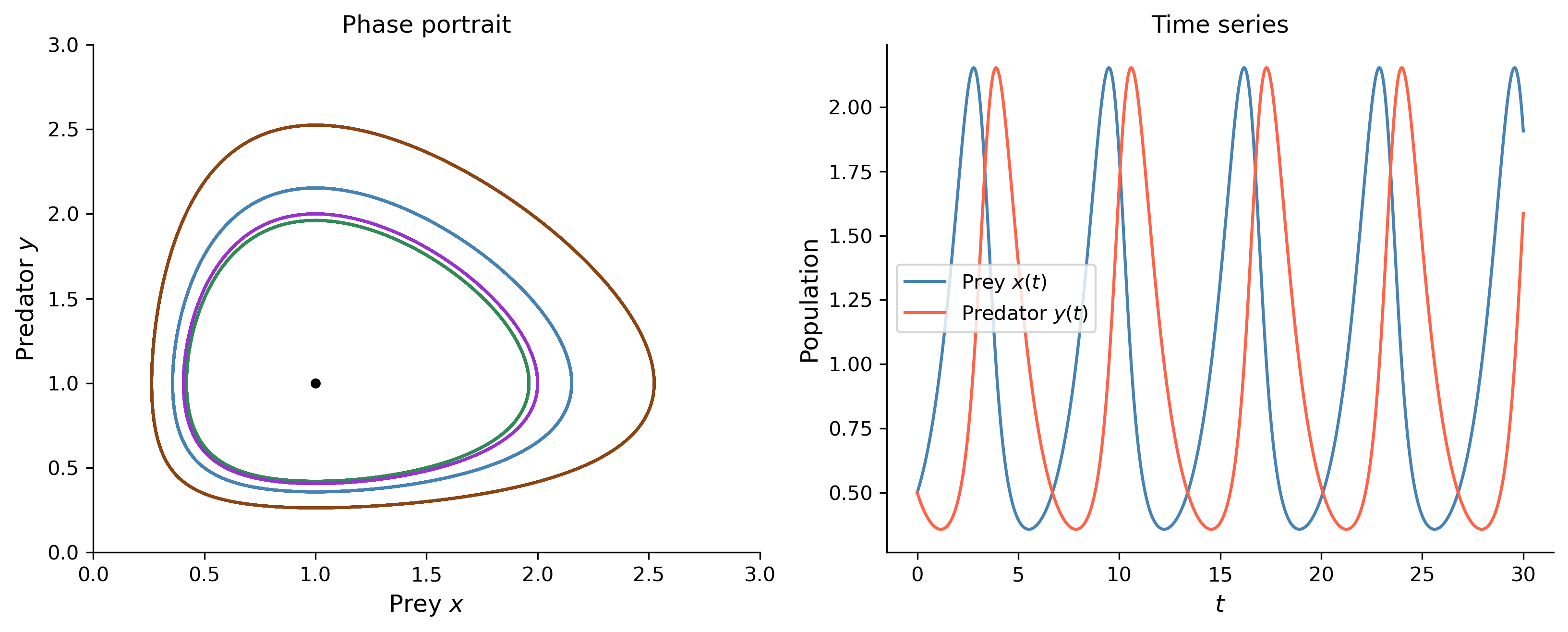
C.9 — The Lotka–Volterra Predator–Prey Model

The classical Lotka–Volterra system (Logan, §5.3.1) models predator ($y$) and prey ($x$) populations: \[ x' = ax - bxy, \qquad y' = -cy + dxy, \] where $a, b, c, d > 0$. The nontrivial equilibrium is $(c/d,\, a/b)$. Solutions are closed orbits around this equilibrium — periodic oscillations — which can be confirmed by a conserved energy-like quantity.

By Hand

Equilibria (with $a=b=c=d=1$): $(0,0)$ (saddle) and $(1,1)$ (center).

Conservation law. Dividing $y'/x' = (-y+xy)/(x-xy)$ and separating: \[ \frac{(-1+x)}{x}\,dx = \frac{(1-y)}{y}\,dy \quad\Longrightarrow\quad \ln x - x + \ln y - y = \text{const}, \] confirming closed orbits.

Phase Portrait and Time Series

Show the code

def lv_rhs(t, y, a=1, b=1, c=1, d=1):
    return [a*y[0] - b*y[0]*y[1],
           -c*y[1] + d*y[0]*y[1]]

t_span = (0, 30)
t_eval = np.linspace(*t_span, 2000)

ics_lv = [(0.5, 0.5), (1.5, 0.5), (0.5, 1.5),
          (2.0, 1.0), (0.3, 1.5)]
colors_lv = ['steelblue', 'tomato', 'seagreen', 'darkorchid', 'saddlebrown']

fig, axes = plt.subplots(1, 2, figsize=(11, 4.5))

for ic, color in zip(ics_lv, colors_lv):
    sol = solve_ivp(lv_rhs, t_span, ic, t_eval=t_eval, rtol=1e-10, atol=1e-12)
    axes[0].plot(sol.y[0], sol.y[1], color=color, lw=1.5)
    if ic == (0.5, 0.5):
        axes[1].plot(sol.t, sol.y[0], color='steelblue', lw=1.5, label='Prey $x(t)$')
        axes[1].plot(sol.t, sol.y[1], color='tomato',    lw=1.5, label='Predator $y(t)$')

axes[0].plot(1, 1, 'k.', ms=8, zorder=5)
axes[0].set_xlabel('Prey $x$',     fontsize=12)
axes[0].set_ylabel('Predator $y$', fontsize=12)
axes[0].set_title('Phase portrait', fontsize=12)
axes[0].set_xlim(0, 3); axes[0].set_ylim(0, 3)

axes[1].set_xlabel(r'$t$',         fontsize=12)
axes[1].set_ylabel('Population',   fontsize=12)
axes[1].set_title('Time series',   fontsize=12)
axes[1].legend(fontsize=10)

plt.tight_layout()
plt.show()

Figure 5: Lotka–Volterra predator–prey dynamics ($a=b=c=d=1$). Left: phase portrait showing closed orbits around the coexistence equilibrium $(1,1)$. Right: time series — prey (blue) and predator (red) oscillate out of phase.

C.10 — Nonlinear Mechanics: The Pendulum

The undamped nonlinear pendulum (Logan, §5.2) obeys \[ \theta'' + \frac{g}{L}\sin\theta = 0, \] or as a system: $\theta' = \omega$, $\omega' = -(g/L)\sin\theta$.

Equilibria: $(\theta, 0)$ with $\sin\theta = 0$, i.e. $\theta = n\pi$.

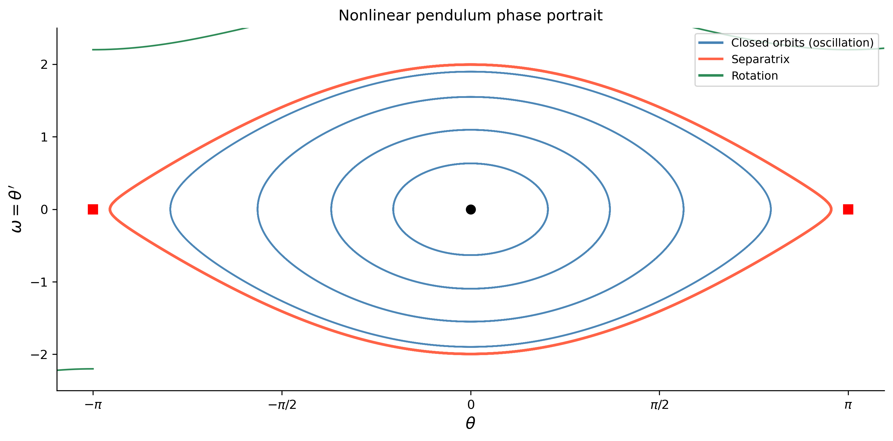
$\theta^* = 0$ (hanging down): Jacobian eigenvalues $\pm i\sqrt{g/L}$ → center.
$\theta^* = \pi$ (balanced up): Jacobian eigenvalues $\pm\sqrt{g/L}$ → saddle.

A conserved energy $E = \frac{1}{2}\omega^2 - \frac{g}{L}\cos\theta$ (constant along trajectories) explains the closed orbits (oscillations) and the separatrix connecting the saddle points (the boundary between oscillation and full rotation).

Phase Portrait

Show the code

gL = 1.0  # g/L

def pendulum_rhs(t, y):
    return [y[1], -gL*np.sin(y[0])]

fig, ax = plt.subplots(figsize=(10, 5))

# Closed orbits (small and moderate amplitude)
for E_val, color in [(-0.8, 'steelblue'), (-0.4, 'steelblue'),
                      (0.2, 'steelblue'),  (0.8, 'steelblue')]:
    # Find theta0 from E = -gL*cos(theta0), omega0=0
    theta0 = np.arccos(-E_val / gL)
    for sign in [1, -1]:
        sol = solve_ivp(pendulum_rhs, (0, 30), [sign*theta0, 0],
                        t_eval=np.linspace(0, 30, 3000), rtol=1e-10)
        ax.plot(sol.y[0], sol.y[1], color=color, lw=1.3, alpha=0.8)

# Separatrix: E = gL  (passes through (pi, 0))
t_sep = np.linspace(0, 10, 3000)
for ic_sep in [(3.0, 0.01), (3.0, -0.01), (-3.0, 0.01), (-3.0, -0.01)]:
    sol_s = solve_ivp(pendulum_rhs, (0, 25), list(ic_sep),
                      t_eval=np.linspace(0, 25, 5000), rtol=1e-12)
    mask = np.abs(sol_s.y[0]) <= np.pi + 0.05
    ax.plot(sol_s.y[0][mask], sol_s.y[1][mask], 'tomato', lw=2.0)

# Rotational solutions outside separatrix
for omega0 in [2.2, -2.2]:
    sol_r = solve_ivp(pendulum_rhs, (0, 15), [-np.pi, omega0],
                      t_eval=np.linspace(0, 15, 2000), rtol=1e-10)
    ax.plot(sol_r.y[0], sol_r.y[1], color='seagreen', lw=1.3)

# Mark equilibria
for x_eq in [-np.pi, 0, np.pi]:
    style = 'rs' if abs(x_eq) > 0.1 else 'ko'
    ax.plot(x_eq, 0, style, ms=7, zorder=5)

ax.set_xlim(-np.pi-0.3, np.pi+0.3)
ax.set_ylim(-2.5, 2.5)
ax.set_xlabel(r'$\theta$', fontsize=13)
ax.set_ylabel(r"$\omega = \theta'$", fontsize=13)
ax.set_title('Nonlinear pendulum phase portrait', fontsize=12)
ax.set_xticks([-np.pi, -np.pi/2, 0, np.pi/2, np.pi])
ax.set_xticklabels([r'$-\pi$', r'$-\pi/2$', r'$0$', r'$\pi/2$', r'$\pi$'])
from matplotlib.lines import Line2D
ax.legend(handles=[
    Line2D([0],[0], color='steelblue', lw=2, label='Closed orbits (oscillation)'),
    Line2D([0],[0], color='tomato',    lw=2, label='Separatrix'),
    Line2D([0],[0], color='seagreen',  lw=2, label='Rotation'),
], fontsize=9, loc='upper right')
plt.tight_layout()
plt.show()

Figure 6: Phase portrait of the nonlinear pendulum ($g/L=1$). Closed orbits (blue) are small-amplitude oscillations. The red **separatrix** passes through the unstable equilibrium $(\pm\pi, 0)$ and separates oscillatory from rotational motion.

C.11 — Population Ecology: Competing Species

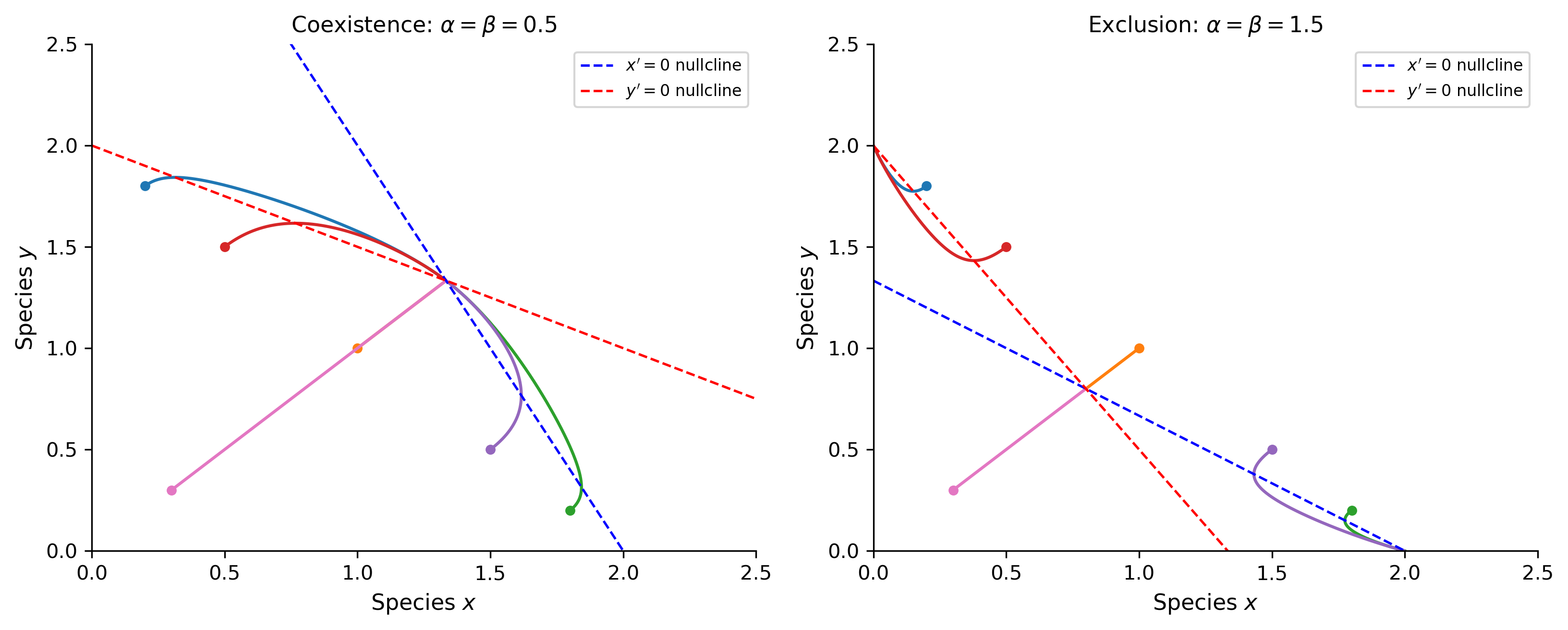
The two-species competition model (Logan, §5.3.2) is \[ x' = r_1 x\!\left(1 - \frac{x + \alpha y}{K_1}\right), \qquad y' = r_2 y\!\left(1 - \frac{y + \beta x}{K_2}\right), \] where $\alpha, \beta$ are competition coefficients. Equilibria include $(0,0)$, $(K_1,0)$, $(0,K_2)$, and potentially a coexistence point. The outcome (which species wins) depends on whether the nullclines intersect inside the positive quadrant and the stability of boundary equilibria.

By Hand (nullcline analysis)

$x$-nullclines ($x'=0$): $x=0$ or $x + \alpha y = K_1$.

$y$-nullclines ($y'=0$): $y=0$ or $\beta x + y = K_2$.

The two non-trivial nullclines intersect at a coexistence equilibrium if and only if the linear system $x + \alpha y = K_1$, $\beta x + y = K_2$ has a solution with $x,y > 0$.

Phase Portrait

Show the code

def comp_rhs(t, y, r1=1, r2=1, K1=2, K2=2, alpha=0.5, beta=0.5):
    x, z = y
    xdot = r1*x*(1 - (x + alpha*z)/K1) if x > 0 else 0
    zdot  = r2*z*(1 - (z + beta*x)/K2)  if z > 0 else 0
    return [xdot, zdot]

fig, axes = plt.subplots(1, 2, figsize=(11, 4.5))

param_sets = [
    dict(alpha=0.5, beta=0.5, title=r'Coexistence: $\alpha=\beta=0.5$'),
    dict(alpha=1.5, beta=1.5, title=r'Exclusion: $\alpha=\beta=1.5$'),
]

ics_comp = [(0.2, 1.8), (1.0, 1.0), (1.8, 0.2),
            (0.5, 1.5), (1.5, 0.5), (0.3, 0.3)]

for ax, params in zip(axes, param_sets):
    rhs_keys = {k: v for k, v in params.items() if k != 'title'}
    rhs = lambda t, y, p=rhs_keys: comp_rhs(t, y, **p)
    colors_c = plt.cm.tab10(np.linspace(0, 0.6, len(ics_comp)))
    for ic, color in zip(ics_comp, colors_c):
        sol = solve_ivp(rhs, (0, 15), list(ic),
                        t_eval=np.linspace(0, 15, 800), rtol=1e-9)
        ax.plot(sol.y[0], sol.y[1], color=color, lw=1.5)
        ax.plot(ic[0], ic[1], 'o', color=color, ms=4)

    # Nullclines
    x_nc = np.linspace(0, 2.5, 200)
    alpha, beta = params['alpha'], params['beta']
    ax.plot(x_nc, (2 - x_nc)/alpha, 'b--', lw=1.2,
            label=r"$x'=0$ nullcline")
    ax.plot(x_nc, 2 - beta*x_nc,     'r--', lw=1.2,
            label=r"$y'=0$ nullcline")
    ax.set_xlim(0, 2.5); ax.set_ylim(0, 2.5)
    ax.set_xlabel('Species $x$', fontsize=11)
    ax.set_ylabel('Species $y$', fontsize=11)
    ax.set_title(params['title'], fontsize=11)
    ax.legend(fontsize=8)

plt.tight_layout()
plt.show()

Figure 7: Competition model phase portraits for two parameter regimes. Left: $\alpha=0.5, \beta=0.5$ (coexistence — stable interior equilibrium). Right: $\alpha=1.5, \beta=1.5$ (competitive exclusion — one species wins depending on initial conditions).

C.12 — The SIR Epidemic Model

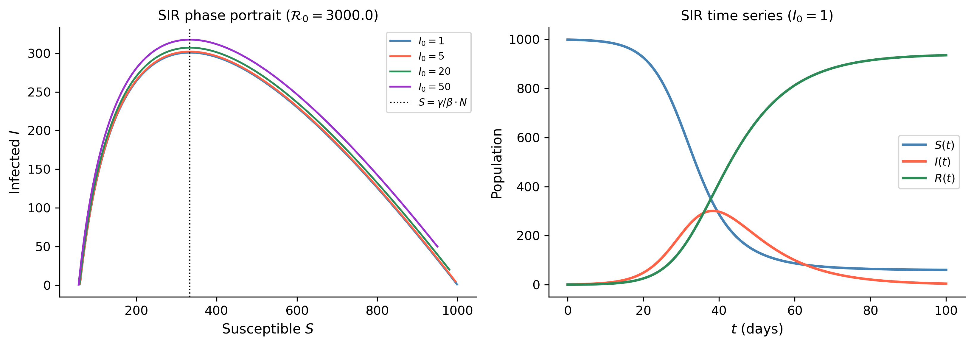
The SIR model (Logan, §5.3.3) tracks Susceptible ($S$), Infected ($I$), and Recovered ($R$) individuals: \[ S' = -\beta SI, \qquad I' = \beta SI - \gamma I, \qquad R' = \gamma I, \] with $N = S + I + R$ constant. Since $R = N - S - I$, only two equations are needed.

Key parameter: basic reproduction number $\mathcal{R}_0 = \beta N/\gamma$.

If $\mathcal{R}_0 \le 1$: epidemic dies out.
If $\mathcal{R}_0 > 1$: epidemic grows initially, peaks when $S = \gamma/\beta$, then declines.

Phase Portrait and Time Series

Show the code

beta_sir, gamma_sir, N_sir = 0.3, 0.1, 1000.0
R0 = beta_sir * N_sir / gamma_sir

def sir_rhs(t, y):
    S, I = y
    return [-beta_sir*S*I/N_sir,
             beta_sir*S*I/N_sir - gamma_sir*I]

t_span_sir = (0, 100)
t_eval_sir = np.linspace(*t_span_sir, 2000)

fig, axes = plt.subplots(1, 2, figsize=(11, 4))

# Phase portrait: vary I0
for I0, color in zip([1, 5, 20, 50], ['steelblue','tomato','seagreen','darkorchid']):
    S0 = N_sir - I0
    sol = solve_ivp(sir_rhs, t_span_sir, [S0, I0],
                    t_eval=t_eval_sir, rtol=1e-10)
    axes[0].plot(sol.y[0], sol.y[1], color=color, lw=1.5,
                 label=f'$I_0={I0}$')

axes[0].axvline(gamma_sir/beta_sir * N_sir, color='k', ls=':', lw=1,
                label=r'$S=\gamma/\beta \cdot N$')
axes[0].set_xlabel('Susceptible $S$', fontsize=11)
axes[0].set_ylabel('Infected $I$',    fontsize=11)
axes[0].set_title(f'SIR phase portrait ($\\mathcal{{R}}_0={R0:.1f}$)', fontsize=11)
axes[0].legend(fontsize=8)

# Time series: I0=1
sol_ts = solve_ivp(sir_rhs, t_span_sir, [N_sir-1, 1],
                   t_eval=t_eval_sir, rtol=1e-10)
axes[1].plot(sol_ts.t, sol_ts.y[0], color='steelblue', lw=2, label='$S(t)$')
axes[1].plot(sol_ts.t, sol_ts.y[1], color='tomato',    lw=2, label='$I(t)$')
axes[1].plot(sol_ts.t, N_sir - sol_ts.y[0] - sol_ts.y[1],
             color='seagreen', lw=2, label='$R(t)$')
axes[1].set_xlabel(r'$t$ (days)',   fontsize=11)
axes[1].set_ylabel('Population',    fontsize=11)
axes[1].set_title('SIR time series ($I_0=1$)', fontsize=11)
axes[1].legend(fontsize=9)

plt.tight_layout()
plt.show()

Figure 8: SIR epidemic model with $\beta=0.3$, $\gamma=0.1$, $N=1000$, giving $\mathcal{R}_0=3$. Left: trajectories in the $(S,I)$ plane for several initial conditions. Right: time series showing the epidemic curve $I(t)$ (red) and $S(t)$ (blue).

Tip

Pattern. For multi-species or compartment models: find equilibria from $\mathbf{f}=\mathbf{0}$, compute $J$ at each, classify. Draw nullclines ($f_i=0$ curves) in the phase plane — their intersections locate equilibria and their geometry reveals which region each trajectory enters.

C.13 — Selected Review Exercises

Exercise C.1 — Full Analysis of a Linear System

Problem. For the system $\mathbf{x}' = \begin{pmatrix}-3&1\\1&-3\end{pmatrix}\mathbf{x}$: (a) find eigenvalues and eigenvectors; (b) write the general solution; (c) classify the equilibrium; (d) solve the IVP with $\mathbf{x}(0) = (2, 0)^T$.

By Hand.

$\lambda^2 + 6\lambda + 8 = (\lambda+2)(\lambda+4) = 0$, so $\lambda_1 = -2$, $\lambda_2 = -4$.

Eigenvectors: $(1,1)^T$ for $\lambda_1 = -2$; $(1,-1)^T$ for $\lambda_2 = -4$.

$(t) = c_1 e^{-2t} \[\begin{pmatrix}1\\1\end{pmatrix}\]

c_2 e^{-4t} \[\begin{pmatrix}1\\-1\end{pmatrix}\] $.

Both eigenvalues negative → stable node.
$c_1 + c_2 = 2$, $c_1 - c_2 = 0$ → $c_1 = c_2 = 1$.

\[ \mathbf{x}(t) = e^{-2t}\begin{pmatrix}1\\1\end{pmatrix} + e^{-4t}\begin{pmatrix}1\\-1\end{pmatrix}. \]

t = sym.Symbol('t')
A_ex1 = sym.Matrix([[-3, 1], [1, -3]])

display(Math(r'A = ' + sym.latex(A_ex1)
             + r',\quad \text{type: } \mathbf{'
             + classify_equilibrium(A_ex1) + r'}'))

x1f, x2f = sym.Function('x1'), sym.Function('x2')
sys_ex1 = [sym.Eq(x1f(t).diff(t), -3*x1f(t) + x2f(t)),
           sym.Eq(x2f(t).diff(t),   x1f(t) - 3*x2f(t))]
sol_ex1 = sym.dsolve(sys_ex1,
                     ics={x1f(0): 2, x2f(0): 0})
for eq in sol_ex1:
    display(Math(sym.latex(sym.simplify(eq))))

$\displaystyle A = \left[\begin{matrix}-3 & 1\\1 & -3\end{matrix}\right],\quad \text{type: } \mathbf{Stable node}$

$\displaystyle x_{1}{\left(t \right)} = \left(e^{2 t} + 1\right) e^{- 4 t}$

$\displaystyle x_{2}{\left(t \right)} = \left(e^{2 t} - 1\right) e^{- 4 t}$

Show the code

def ex1_rhs(t, y):
    return [-3*y[0]+y[1], y[0]-3*y[1]]

fig, ax = plt.subplots(figsize=(6, 5))
x1g = np.linspace(-3, 3, 22)
X1c, X2c = np.meshgrid(x1g, x1g)
dX1c = -3*X1c + X2c
dX2c =  X1c - 3*X2c
speed = np.sqrt(dX1c**2+dX2c**2); speed[speed==0]=1
ax.streamplot(X1c, X2c, dX1c/speed, dX2c/speed,
              density=1.0, color='lightgray', linewidth=0.8)

ics_ex1 = [(2,0),(0,2),(-2,0),(0,-2),(2,2),(-2,-2)]
for ic in ics_ex1:
    sol = solve_ivp(ex1_rhs, (0, 3), list(ic),
                    t_eval=np.linspace(0, 3, 400), rtol=1e-9)
    ax.plot(sol.y[0], sol.y[1], 'steelblue', lw=1.8)

# Eigendirections
for v, ls in [([1,1],'--'), ([1,-1],':')]:
    nv = np.array(v)/np.linalg.norm(v)
    ax.plot([-3*nv[0],3*nv[0]], [-3*nv[1],3*nv[1]],
            'k', ls=ls, lw=1.4)

ax.set_xlim(-3,3); ax.set_ylim(-3,3)
ax.axhline(0,color='k',lw=0.4); ax.axvline(0,color='k',lw=0.4)
ax.set_xlabel(r'$x_1$',fontsize=12); ax.set_ylabel(r'$x_2$',fontsize=12)
ax.set_title('Stable node', fontsize=12)
ax.set_aspect('equal')
plt.tight_layout()
plt.show()

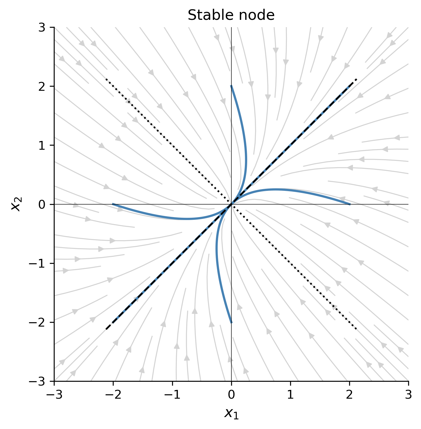
Figure 9: Phase portrait for Exercise C.1. The origin is a **stable node**; all trajectories approach it along the slow eigendirection $\mathbf{v}_1=(1,1)^T$ ($\lambda_1=-2$), with the fast component ($\lambda_2=-4$) decaying first.

Exercise C.2 — Nonlinear System: Full Analysis

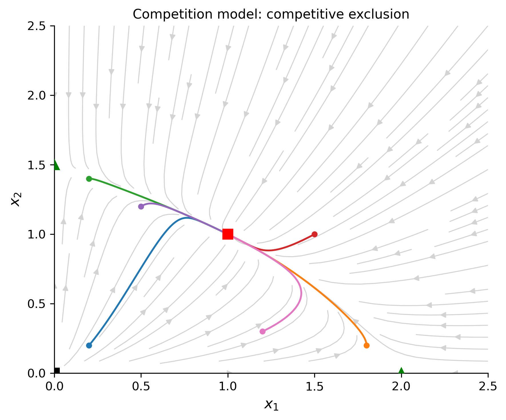
Problem. Analyze all equilibria of the nonlinear system \[ x_1' = x_1(2 - x_1 - x_2), \qquad x_2' = x_2(3 - x_1 - 2x_2). \] (This is a competition model with $K_1=2$, $K_2=3/2$, $\alpha=\beta=1$.)

Equilibria. Setting $f_1 = f_2 = 0$:

$(0,0)$: trivial
$(2,0)$: prey-only
$(0, 3/2)$: competitor-only
Solve $x_1 + x_2 = 2$ and $x_1 + 2x_2 = 3$: $x_2 = 1$, $x_1 = 1$ → $(1,1)$.

x1, x2 = sym.symbols('x1 x2', nonnegative=True)

f1_nl = x1*(2 - x1 - x2)
f2_nl = x2*(3 - x1 - 2*x2)

F_nl = sym.Matrix([f1_nl, f2_nl])
J_nl = F_nl.jacobian(sym.Matrix([x1, x2]))

equil_nl = sym.solve([f1_nl, f2_nl], [x1, x2], dict=True)
print("Equilibria:")
for eq in equil_nl:
    J_at = J_nl.subs(eq)
    etype = classify_equilibrium(J_at)
    evals = list(J_at.eigenvals().keys())
    display(Math(r'\mathbf{x}^* = '
                 + sym.latex(sym.Matrix([eq[x1], eq[x2]]))
                 + r',\quad \lambda = ' + sym.latex(evals)
                 + r'\quad\Rightarrow\quad \text{' + etype + '}'))

Equilibria:

$\displaystyle \mathbf{x}^* = \left[\begin{matrix}0\\0\end{matrix}\right],\quad \lambda = \left[ 2, \ 3\right]\quad\Rightarrow\quad \text{Unstable node}$

$\displaystyle \mathbf{x}^* = \left[\begin{matrix}0\\\frac{3}{2}\end{matrix}\right],\quad \lambda = \left[ \frac{1}{2}, \ -3\right]\quad\Rightarrow\quad \text{Saddle}$

$\displaystyle \mathbf{x}^* = \left[\begin{matrix}1\\1\end{matrix}\right],\quad \lambda = \left[ - \frac{3}{2} - \frac{\sqrt{5}}{2}, \ - \frac{3}{2} + \frac{\sqrt{5}}{2}\right]\quad\Rightarrow\quad \text{Stable node}$

$\displaystyle \mathbf{x}^* = \left[\begin{matrix}2\\0\end{matrix}\right],\quad \lambda = \left[ 1, \ -2\right]\quad\Rightarrow\quad \text{Saddle}$

Show the code

def nl_rhs(t, y):
    x, z = max(y[0], 0), max(y[1], 0)
    return [x*(2 - x - z), z*(3 - x - 2*z)]

fig, ax = plt.subplots(figsize=(6, 5))
x1g = np.linspace(0, 2.5, 24)
X1c, X2c = np.meshgrid(x1g, np.linspace(0, 2.5, 24))
dX1c = X1c*(2 - X1c - X2c)
dX2c = X2c*(3 - X1c - 2*X2c)
spd  = np.sqrt(dX1c**2+dX2c**2); spd[spd==0]=1
ax.streamplot(X1c, X2c, dX1c/spd, dX2c/spd,
              density=1.0, color='lightgray', linewidth=0.8)

ics_nl = [(0.2, 0.2), (1.8, 0.2), (0.2, 1.4),
          (1.5, 1.0), (0.5, 1.2), (1.2, 0.3)]
colors_nl = plt.cm.tab10(np.linspace(0, 0.6, len(ics_nl)))
for ic, col in zip(ics_nl, colors_nl):
    sol = solve_ivp(nl_rhs, (0, 20), list(ic),
                    t_eval=np.linspace(0, 20, 800), rtol=1e-9)
    ax.plot(sol.y[0], sol.y[1], color=col, lw=1.5)
    ax.plot(ic[0], ic[1], 'o', color=col, ms=4)

for (xe, ye), mk in [((0,0),'ks'),((2,0),'g^'),((0,1.5),'g^'),((1,1),'rs')]:
    ax.plot(xe, ye, mk, ms=8, zorder=6)

ax.set_xlim(0,2.5); ax.set_ylim(0,2.5)
ax.set_xlabel(r'$x_1$',fontsize=12); ax.set_ylabel(r'$x_2$',fontsize=12)
ax.set_title('Competition model: competitive exclusion', fontsize=11)
plt.tight_layout()
plt.show()

Figure 10: Phase portrait for the competition model in Exercise C.2. The coexistence equilibrium $(1,1)$ is a saddle — competitive exclusion occurs. Trajectories go to either $(2,0)$ or $(0,3/2)$ depending on initial conditions.

Exercise C.3 — Numerical Exploration: Chaos in the Lorenz System

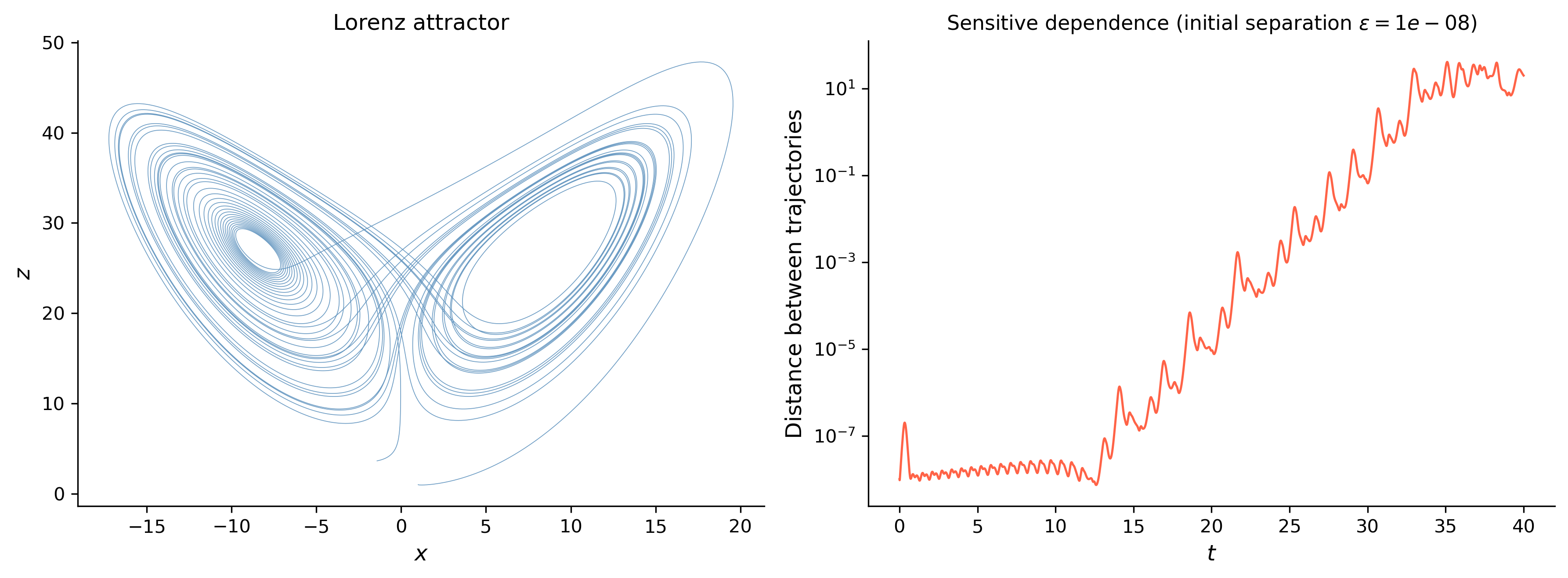
As a capstone, we explore the Lorenz system (a famous nonlinear 3D system), which exhibits sensitive dependence on initial conditions — the hallmark of chaos. While beyond Logan’s scope, it illustrates the power of solve_ivp for nonlinear systems: \[ x' = \sigma(y - x), \quad y' = x(\rho - z) - y, \quad z' = xy - \beta z, \] with $\sigma = 10$, $\rho = 28$, $\beta = 8/3$.

Show the code

def lorenz(t, y, sigma=10, rho=28, beta=8/3):
    x, yy, z = y
    return [sigma*(yy-x), x*(rho-z)-yy, x*yy - beta*z]

t_lor  = np.linspace(0, 40, 20000)
eps    = 1e-8
ic1    = [1.0, 1.0, 1.0]
ic2    = [1.0 + eps, 1.0, 1.0]

sol_l1 = solve_ivp(lorenz, (0, 40), ic1, t_eval=t_lor, rtol=1e-10, atol=1e-12)
sol_l2 = solve_ivp(lorenz, (0, 40), ic2, t_eval=t_lor, rtol=1e-10, atol=1e-12)

fig, axes = plt.subplots(1, 2, figsize=(12, 4.5))

axes[0].plot(sol_l1.y[0], sol_l1.y[2], color='steelblue', lw=0.4, alpha=0.8)
axes[0].set_xlabel(r'$x$', fontsize=12)
axes[0].set_ylabel(r'$z$', fontsize=12)
axes[0].set_title('Lorenz attractor', fontsize=12)

dist = np.sqrt((sol_l1.y[0]-sol_l2.y[0])**2
              +(sol_l1.y[1]-sol_l2.y[1])**2
              +(sol_l1.y[2]-sol_l2.y[2])**2)
axes[1].semilogy(sol_l1.t, dist, color='tomato', lw=1.2)
axes[1].set_xlabel(r'$t$', fontsize=12)
axes[1].set_ylabel('Distance between trajectories', fontsize=12)
axes[1].set_title(f'Sensitive dependence (initial separation $\\varepsilon={eps}$)',
                  fontsize=11)

plt.tight_layout()
plt.show()

Figure 11: The Lorenz attractor ($\sigma=10, \rho=28, \beta=8/3$). Left: the butterfly-shaped attractor in the $(x,z)$-plane. Right: two trajectories with nearly identical initial conditions (difference $10^{-8}$) diverge exponentially — sensitive dependence, the signature of chaos.

C.14 — Summary: Systems Analysis Toolkit

The table below collects the key steps for analyzing a $2\times2$ system — linear or nonlinear.

Step	Linear $\mathbf{x}'=A\mathbf{x}$	Nonlinear $\mathbf{x}'=\mathbf{f}(\mathbf{x})$
1. Find equilibria	Only $(0,0)$	Solve $\mathbf{f}=\mathbf{0}$
2. Characteristic equation	$\det(A-\lambda I)=0$	$\det(J-\lambda I)=0$ at each $\mathbf{x}^*$
3. Classify	Table from $\tau, \Delta$	Same table (if hyperbolic)
4. General solution	$c_1 e^{\lambda_1 t}\mathbf{v}_1 + c_2 e^{\lambda_2 t}\mathbf{v}_2$	No formula; use `solve_ivp`
5. Phase portrait	Straight-line eigendirections	Draw nullclines; use `solve_ivp`

# Convenience wrapper: full analysis of any 2x2 matrix
def analyze_system(A_mat, label=""):
    tr  = sym.simplify(A_mat.trace())
    det = sym.simplify(A_mat.det())
    cp  = sym.factor(A_mat.charpoly().as_expr())
    evs = list(A_mat.eigenvals().keys())
    et  = classify_equilibrium(A_mat)
    display(Math((label + r': ' if label else '')
                 + r'A=' + sym.latex(A_mat)
                 + r',\; \tau=' + sym.latex(tr)
                 + r',\; \Delta=' + sym.latex(det)
                 + r',\; p(\lambda)=' + sym.latex(cp)
                 + r',\; \lambda=' + sym.latex(evs)
                 + r'\;\Rightarrow\;\text{' + et + '}'))

matrices_to_check = [
    (sym.Matrix([[2, 1],[-1, 2]]),  "Unstable spiral"),
    (sym.Matrix([[-2,-1],[1,-2]]), "Stable spiral"),
    (sym.Matrix([[0,-3],[3, 0]]),  "Center"),
    (sym.Matrix([[1, 0],[0,-1]]),  "Saddle"),
    (sym.Matrix([[-2,0],[0,-5]]),  "Stable node"),
]
for M, lbl in matrices_to_check:
    analyze_system(M, lbl)

$\displaystyle Unstable spiral: A=\left[\begin{matrix}2 & 1\\-1 & 2\end{matrix}\right],\; \tau=4,\; \Delta=5,\; p(\lambda)=\lambda^{2} - 4 \lambda + 5,\; \lambda=\left[ 2 - i, \ 2 + i\right]\;\Rightarrow\;\text{Unstable spiral}$

$\displaystyle Stable spiral: A=\left[\begin{matrix}-2 & -1\\1 & -2\end{matrix}\right],\; \tau=-4,\; \Delta=5,\; p(\lambda)=\lambda^{2} + 4 \lambda + 5,\; \lambda=\left[ -2 - i, \ -2 + i\right]\;\Rightarrow\;\text{Stable spiral}$

$\displaystyle Center: A=\left[\begin{matrix}0 & -3\\3 & 0\end{matrix}\right],\; \tau=0,\; \Delta=9,\; p(\lambda)=\lambda^{2} + 9,\; \lambda=\left[ - 3 i, \ 3 i\right]\;\Rightarrow\;\text{Center}$

$\displaystyle Saddle: A=\left[\begin{matrix}1 & 0\\0 & -1\end{matrix}\right],\; \tau=0,\; \Delta=-1,\; p(\lambda)=\left(\lambda - 1\right) \left(\lambda + 1\right),\; \lambda=\left[ 1, \ -1\right]\;\Rightarrow\;\text{Saddle}$

$\displaystyle Stable node: A=\left[\begin{matrix}-2 & 0\\0 & -5\end{matrix}\right],\; \tau=-7,\; \Delta=10,\; p(\lambda)=\left(\lambda + 2\right) \left(\lambda + 5\right),\; \lambda=\left[ -2, \ -5\right]\;\Rightarrow\;\text{Stable node}$

References

Logan, J David. 2015. A First Course in Differential Equations, Third Edition.

Expand for Session Info

import sys, importlib
print("Python version:", sys.version)
for name in ['numpy', 'sympy', 'scipy', 'matplotlib']:
    mod = importlib.import_module(name)
    print(f"{name}=={mod.__version__}")

Python version: 3.14.4 | packaged by conda-forge | (main, Apr  8 2026, 02:33:53) [Clang 20.1.8 ]
numpy==2.4.3
sympy==1.14.0
scipy==1.17.1
matplotlib==3.10.8

Reuse

CC BY-NC-SA 4.0

Region in \((\Delta, \tau)\)-plane	Equilibrium type
\(\Delta < 0\)	Saddle
\(\Delta > 0\), \(\tau^2 - 4\Delta > 0\), \(\tau < 0\)	Stable node
\(\Delta > 0\), \(\tau^2 - 4\Delta > 0\), \(\tau > 0\)	Unstable node
\(\Delta > 0\), \(\tau^2 - 4\Delta < 0\), \(\tau < 0\)	Stable spiral
\(\Delta > 0\), \(\tau^2 - 4\Delta < 0\), \(\tau > 0\)	Unstable spiral
\(\Delta > 0\), \(\tau = 0\)	Center