Review — Laplace Transforms

Show the code

# Imports for the entire session
import numpy as np                         # NumPy for numerical computations
import sympy as sym                        # SymPy for symbolic mathematics
import matplotlib as mpl                   # Matplotlib for plotting
import matplotlib.pyplot as plt            # Matplotlib pyplot interface
from scipy.integrate import solve_ivp      # SciPy numerical ODE solver
from IPython.display import Math, display
mpl.rcParams['figure.dpi'] = 150
mpl.rcParams['axes.spines.top'] = False
mpl.rcParams['axes.spines.right'] = False

This document reviews the Laplace transform methods covered in Chapter 3 of (Logan 2015). It is structured as a companion to Appendix A of the text (reviewed in Review 1): each section states the key idea, works through a representative example by hand, and then demonstrates the same calculation using Python — primarily SymPy for symbolic transforms and SciPy/Matplotlib for numerical simulation and visualization.

The central idea of the chapter is this:

The Laplace transform turns derivative operations in the time domain into multiplication operations in the transform domain.

This converts an initial value problem for a differential equation into an algebraic problem for the transformed state function \(X(s)\), which we solve and then invert.

B.1 — Definition and Basic Transforms

Definition (Logan, §3.1). Let \(x = x(t)\) be defined on \(0 \le t < \infty\). The Laplace transform of \(x(t)\) is \[ X(s) = \mathcal{L}[x(t)](s) = \int_0^\infty x(t)\,e^{-st}\,dt, \] provided the improper integral converges. The transform is a linear operator: \[ \mathcal{L}[\alpha x + \beta y] = \alpha\mathcal{L}[x] + \beta\mathcal{L}[y]. \]

The three most fundamental transforms, derived directly from the definition, are

\(x(t)\)	\(X(s) = \mathcal{L}[x]\)	Condition
\(e^{at}\)	\(\dfrac{1}{s-a}\)	\(s > a\)
\(1\)	\(\dfrac{1}{s}\)	\(s > 0\)
\(t\)	\(\dfrac{1}{s^2}\)	\(s > 0\)

By Hand

Example. Compute \(\mathcal{L}[e^{at}]\) from the definition (Logan, Example 3.3).

\[ X(s) = \int_0^\infty e^{at} e^{-st}\,dt = \int_0^\infty e^{(a-s)t}\,dt = \frac{1}{a-s}\,e^{(a-s)t}\Big|_0^\infty = \frac{1}{s-a}, \quad s > a. \]

Example. Compute \(\mathcal{L}[t^n]\) for non-negative integers \(n\) (Logan, Example 3.12).

Use the derivative formula \(\mathcal{L}[x'] = s\mathcal{L}[x] - x(0)\) on \(x(t) = t^n\). Since \((t^n)' = nt^{n-1}\), we get the recurrence \(\mathcal{L}[t^n] = \tfrac{n}{s}\mathcal{L}[t^{n-1}]\). Applying repeatedly from \(\mathcal{L}[1] = 1/s\): \[ \mathcal{L}[t^n] = \frac{n!}{s^{n+1}}, \quad s > 0. \]

Using SymPy

SymPy computes Laplace transforms with sym.laplace_transform and inverse transforms with sym.inverse_laplace_transform.

t, s, a = sym.symbols('t s a', real=True)

# Direct computation from definition via sym.laplace_transform
# Returns (F(s), convergence_plane, condition)
funcs = {
    'e^{at}'  : sym.exp(a*t),
    '1'       : sym.Integer(1),
    't'       : t,
    't^2'     : t**2,
    't^n (n=4)': t**4,
    r'\sin kt': sym.sin(sym.Symbol('k')*t),
    r'\cos kt': sym.cos(sym.Symbol('k')*t),
    r'\sinh kt': sym.sinh(sym.Symbol('k')*t),
    r'\cosh kt': sym.cosh(sym.Symbol('k')*t),
}

for name, f in funcs.items():
    F, plane, cond = sym.laplace_transform(f, t, s, noconds=False)
    display(Math(
        r'\mathcal{L}\!\left[' + name + r'\right] = '
        + sym.latex(sym.simplify(F))
        + r'\quad (' + sym.latex(cond) + r')'
    ))

\(\displaystyle \mathcal{L}\!\left[e^{at}\right] = \frac{1}{- a + s}\quad (\text{True})\)

\(\displaystyle \mathcal{L}\!\left[1\right] = \frac{1}{s}\quad (\text{True})\)

\(\displaystyle \mathcal{L}\!\left[t\right] = \frac{1}{s^{2}}\quad (\text{True})\)

\(\displaystyle \mathcal{L}\!\left[t^2\right] = \frac{2}{s^{3}}\quad (\text{True})\)

\(\displaystyle \mathcal{L}\!\left[t^n (n=4)\right] = \frac{24}{s^{5}}\quad (\text{True})\)

\(\displaystyle \mathcal{L}\!\left[\sin kt\right] = \frac{k}{k^{2} + s^{2}}\quad (\text{True})\)

\(\displaystyle \mathcal{L}\!\left[\cos kt\right] = \frac{s}{k^{2} + s^{2}}\quad (\text{True})\)

\(\displaystyle \mathcal{L}\!\left[\sinh kt\right] = \frac{k}{- k^{2} + s^{2}}\quad (\text{True})\)

\(\displaystyle \mathcal{L}\!\left[\cosh kt\right] = \frac{s}{- k^{2} + s^{2}}\quad (\text{True})\)

Tip

Pattern. To compute \(\mathcal{L}[x(t)]\) by hand, evaluate the improper integral \(\int_0^\infty x(t)e^{-st}\,dt\) directly, or use the recurrence relation for \(t^n\). In Python, sym.laplace_transform(f, t, s) does this symbolically.

B.2 — Operational Properties

Two additional properties are essential for solving differential equations with discontinuous or shifted inputs.

(a) Shift property (Logan, §3.1, eq. 3.4). Multiplying \(x(t)\) by \(e^{at}\) shifts the transform variable: \[ \mathcal{L}[x(t)\,e^{at}] = X(s - a). \]

(b) Switching property (Logan, §3.1, eq. 3.5). The Heaviside function \(H(t-a)\) acts as a switch that is off for \(t < a\) and on for \(t \ge a\): \[ \mathcal{L}[H(t-a)\,x(t-a)] = e^{-as} X(s). \] In inverse form: \(\mathcal{L}^{-1}[e^{-as} X(s)] = H(t-a)\,x(t-a)\).

The transform of derivatives (Logan, Theorem 3.11) converts the IVP into algebra: \[ \mathcal{L}[x'] = s X(s) - x(0), \qquad \mathcal{L}[x''] = s^2 X(s) - s\,x(0) - x'(0). \]

By Hand

Example. Find \(\mathcal{L}[\cosh t]\) using the derivative formula (Logan, Example 3.13).

Since \((\cosh t)'' = \cosh t\), write \[ \mathcal{L}[(\cosh t)''] = s^2\mathcal{L}[\cosh t] - s\cosh 0 - \sinh 0 = s^2\mathcal{L}[\cosh t] - s. \] But also \(\mathcal{L}[(\cosh t)''] = \mathcal{L}[\cosh t]\). Setting these equal: \[ \mathcal{L}[\cosh t] = s^2\mathcal{L}[\cosh t] - s \quad\Longrightarrow\quad \mathcal{L}[\cosh t] = \frac{s}{s^2 - 1}. \]

Example. Find \(\mathcal{L}[t e^{-2t}]\) using the shift property (Logan, Example 3.9).

We know \(\mathcal{L}[t] = 1/s^2\). Replacing \(s\) with \(s - (-2) = s + 2\): \[ \mathcal{L}[t e^{-2t}] = \frac{1}{(s+2)^2}. \]

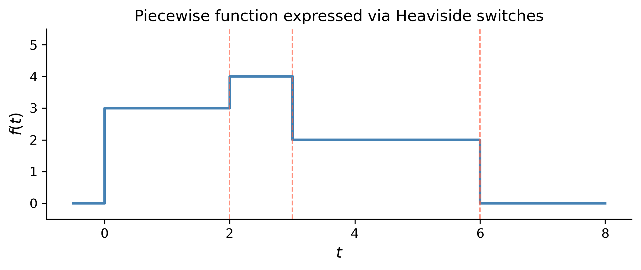
Example. Represent the piecewise function (Logan, Example 3.8) \[ f(t) = \begin{cases} 3, & 0 \le t < 2 \\ 4, & 2 \le t \le 3 \\ 2, & 3 < t \le 6 \\ 0, & t > 6 \end{cases} \] in one line and find \(F(s)\).

Switch on/off with Heaviside functions: \[ f(t) = 3H(t) + H(t-2) - 2H(t-3) - 2H(t-6). \] By linearity and \(\mathcal{L}[H(t-a)] = e^{-as}/s\): \[ F(s) = \frac{3}{s} + \frac{1}{s}e^{-2s} - \frac{2}{s}e^{-3s} - \frac{2}{s}e^{-6s}. \]

Using SymPy

t, s = sym.symbols('t s', real=True, positive=True)
k    = sym.Symbol('k', positive=True)
a    = sym.Symbol('a', positive=True)

# (a) Shift property: L[t * exp(-2t)]
f1 = t * sym.exp(-2*t)
F1, *_ = sym.laplace_transform(f1, t, s, noconds=False)
display(Math(r'\mathcal{L}[t\,e^{-2t}] = ' + sym.latex(F1)))

# (b) Derivative formula: L[cosh t]
f2 = sym.cosh(t)
F2, *_ = sym.laplace_transform(f2, t, s, noconds=False)
display(Math(r'\mathcal{L}[\cosh t] = ' + sym.latex(sym.simplify(F2))))

# (c) Heaviside / switching: the piecewise function from Example 3.8
f3 = (3*sym.Heaviside(t)
      + sym.Heaviside(t-2)
      - 2*sym.Heaviside(t-3)
      - 2*sym.Heaviside(t-6))
F3, *_ = sym.laplace_transform(f3, t, s, noconds=False)
display(Math(r'F(s) = ' + sym.latex(sym.simplify(F3))))

\(\displaystyle \mathcal{L}[t\,e^{-2t}] = \frac{1}{\left(s + 2\right)^{2}}\)

\(\displaystyle \mathcal{L}[\cosh t] = \frac{s}{s^{2} - 1}\)

\(\displaystyle F(s) = \frac{\left(3 e^{6 s} + e^{4 s} - 2 e^{3 s} - 2\right) e^{- 6 s}}{s}\)

Show the code

t_vals = np.linspace(-0.5, 8, 1000)

def f_piece(t):
    return (3*(t >= 0) + 1*(t >= 2) - 2*(t >= 3) - 2*(t >= 6)).astype(float)

fig, ax = plt.subplots(figsize=(7, 3))
ax.step(t_vals, f_piece(t_vals), where='post', color='steelblue', lw=2)
ax.set_xlabel(r'$t$', fontsize=12)
ax.set_ylabel(r'$f(t)$', fontsize=12)
ax.set_title('Piecewise function expressed via Heaviside switches', fontsize=12)
ax.set_ylim(-0.5, 5.5)
for x_loc in [2, 3, 6]:
    ax.axvline(x_loc, color='tomato', ls='--', lw=1, alpha=0.7)
plt.tight_layout()
plt.show()

Figure 1: The piecewise function from Logan Example 3.8, expressed compactly using Heaviside step functions.

Tip

Pattern. The shift property replaces \(s\) by \(s - a\) in the transform. The switching property multiplies \(X(s)\) by \(e^{-as}\) and wraps the time-domain answer in \(H(t-a)\). An exponential factor \(e^{-as}\) in a transform always signals a time delay of \(a\) units.

B.3 — Inverse Transforms and Partial Fractions

The inverse Laplace transform \(\mathcal{L}^{-1}[X(s)] = x(t)\) reverses the process. It is also linear: \[ \mathcal{L}^{-1}[\alpha X + \beta Y] = \alpha\,\mathcal{L}^{-1}[X] + \beta\,\mathcal{L}^{-1}[Y]. \] The key technique for inverting rational functions is partial fractions: decompose \(X(s)\) into simpler terms that appear in the transform table.

By Hand

Example. Invert \(X(s) = \dfrac{1}{(s+1)(s+2)}\) (Logan, Example 3.16).

Partial fractions: \(\dfrac{1}{(s+1)(s+2)} = \dfrac{1}{s+1} - \dfrac{1}{s+2}\).

Therefore \(x(t) = e^{-t} - e^{-2t}\).

Example. Invert \(X(s) = \dfrac{1}{s^2 + 3s + 6}\) (Logan, Example 3.17).

Complete the square in the denominator: \[ s^2 + 3s + 6 = \left(s + \tfrac{3}{2}\right)^2 + \frac{15}{4}. \] So \[ X(s) = \frac{1}{\left(s + \frac{3}{2}\right)^2 + \left(\frac{\sqrt{15}}{2}\right)^2}. \] From the table, \(\mathcal{L}^{-1}\!\left[\dfrac{k}{(s-a)^2+k^2}\right] = e^{at}\sin kt\). Here \(a = -3/2\), \(k = \sqrt{15}/2\), so multiply and divide by \(\sqrt{15}/2\): \[ x(t) = \frac{2}{\sqrt{15}}\,e^{-3t/2}\sin\frac{\sqrt{15}}{2}\,t. \]

Example. Invert \(X(s) = \dfrac{e^{-3s}}{s-2}\) (Logan, Example 3.10).

The exponential signals the switching property with \(a = 3\). Since \(\mathcal{L}^{-1}[1/(s-2)] = e^{2t}\): \[ x(t) = H(t-3)\,e^{2(t-3)}. \]

Using SymPy

t, s = sym.symbols('t s', positive=True)

# Example 1: partial fractions
X1 = 1 / ((s+1)*(s+2))
x1 = sym.inverse_laplace_transform(X1, s, t)
display(Math(r'\mathcal{L}^{-1}\!\left[\frac{1}{(s+1)(s+2)}\right] = '
             + sym.latex(sym.simplify(x1))))

# Example 2: complete the square
X2 = 1 / (s**2 + 3*s + 6)
x2 = sym.inverse_laplace_transform(X2, s, t)
display(Math(r'\mathcal{L}^{-1}\!\left[\frac{1}{s^2+3s+6}\right] = '
             + sym.latex(sym.simplify(x2))))

# Example 3: switching property with exponential
X3 = sym.exp(-3*s) / (s - 2)
x3 = sym.inverse_laplace_transform(X3, s, t)
display(Math(r'\mathcal{L}^{-1}\!\left[\frac{e^{-3s}}{s-2}\right] = '
             + sym.latex(sym.simplify(x3))))

\(\displaystyle \mathcal{L}^{-1}\!\left[\frac{1}{(s+1)(s+2)}\right] = \left(e^{t} - 1\right) e^{- 2 t}\)

\(\displaystyle \mathcal{L}^{-1}\!\left[\frac{1}{s^2+3s+6}\right] = \frac{2 \sqrt{15} e^{- \frac{3 t}{2}} \sin{\left(\frac{\sqrt{15} t}{2} \right)}}{15}\)

\(\displaystyle \mathcal{L}^{-1}\!\left[\frac{e^{-3s}}{s-2}\right] = e^{2 t - 6} \theta\left(t - 3\right)\)

Tip

Pattern. To invert \(X(s)\): (1) look for exponential factors \(e^{-as}\) (switching property); (2) factor or complete the square in the denominator; (3) decompose by partial fractions into table entries.

B.4 — Solving Initial Value Problems

The three-step procedure (Logan, §3.2.1):

Transform — take \(\mathcal{L}\) of each term; use Theorem 3.11 to replace derivatives by algebra; initial conditions enter automatically.
Solve — solve the resulting algebraic equation for \(X(s)\).
Invert — apply \(\mathcal{L}^{-1}\) to recover \(x(t)\).

By Hand

Example. Solve \(x'' + k^2 x = 0\), \(x(0) = 0\), \(x'(0) = 1\) (Logan, Example 3.14).

Step 1 — Transform. \[ s^2 X(s) - s\cdot 0 - 1 + k^2 X(s) = 0. \]

Step 2 — Solve for \(X(s)\). \[ X(s)(s^2 + k^2) = 1 \quad\Longrightarrow\quad X(s) = \frac{1}{s^2+k^2} = \frac{1}{k}\cdot\frac{k}{s^2+k^2}. \]

Step 3 — Invert. \[ \boxed{x(t) = \frac{1}{k}\sin kt.} \]

Example. Solve \(x' + 2x = e^{-t}\), \(x(0) = 0\) (Logan, Example 3.15).

Step 1. \(sX - 0 + 2X = \dfrac{1}{s+1}\).

Step 2. \(X(s) = \dfrac{1}{(s+1)(s+2)}\).

Step 3. Partial fractions: \(\dfrac{1}{(s+1)(s+2)} = \dfrac{1}{s+1} - \dfrac{1}{s+2}\).

\[ \boxed{x(t) = e^{-t} - e^{-2t}.} \]

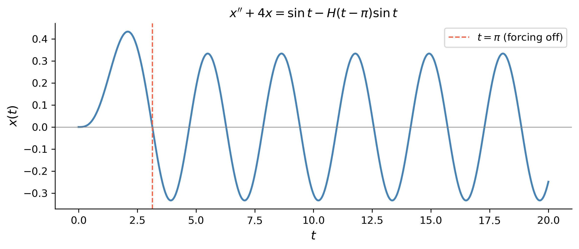
Example. Solve \(x'' + 4x = \sin t - H(t-\pi)\sin t\), \(x(0) = x'(0) = 0\) (Logan, Example 3.19).

Step 1. Using \(\mathcal{L}[H(t-\pi)\sin t] = -e^{-\pi s}/(s^2+1)\): \[ (s^2+4)X(s) = \frac{1}{s^2+1} + \frac{e^{-\pi s}}{s^2+1}. \]

Step 2. \(X(s) = \dfrac{1}{(s^2+1)(s^2+4)} + e^{-\pi s}\dfrac{1}{(s^2+1)(s^2+4)}\).

Step 3. Partial fractions: \(\dfrac{1}{(s^2+1)(s^2+4)} = \dfrac{1/3}{s^2+1} - \dfrac{1/3}{s^2+4}\).

Inverting and applying the switching property: \[ \boxed{x(t) = \frac{1}{3}\sin t - \frac{1}{6}\sin 2t + H(t-\pi)\!\left(\frac{1}{3}\sin(t-\pi) - \frac{1}{6}\sin 2(t-\pi)\right).} \]

Using SymPy

t, s = sym.symbols('t s', positive=True)
x    = sym.Function('x')

# Example 1: x'' + k^2 x = 0, x(0)=0, x'(0)=1
k = sym.Symbol('k', positive=True)
ode1 = sym.Eq(x(t).diff(t,2) + k**2 * x(t), 0)
sol1 = sym.dsolve(ode1, x(t), ics={x(0): 0, x(t).diff(t).subs(t,0): 1})
display(Math(r'\text{Ex 1: }' + sym.latex(sol1)))

# Example 2: x' + 2x = e^{-t}, x(0)=0
ode2 = sym.Eq(x(t).diff(t) + 2*x(t), sym.exp(-t))
sol2 = sym.dsolve(ode2, x(t), ics={x(0): 0})
display(Math(r'\text{Ex 2: }' + sym.latex(sym.simplify(sol2))))

# Example 3: x'' + 4x = sin(t) - H(t-pi)sin(t), x(0)=x'(0)=0
# Use Laplace transforms directly in SymPy
X = sym.Function('X')
# Build X(s) by hand (dsolve struggles with Heaviside forcing)
X_s = (1 + sym.exp(-sym.pi*s)) / ((s**2+1)*(s**2+4))
x3  = sym.inverse_laplace_transform(X_s, s, t)
display(Math(r'\text{Ex 3: } x(t) = ' + sym.latex(sym.simplify(x3))))

\(\displaystyle \text{Ex 1: }x{\left(t \right)} = \frac{\sin{\left(k t \right)}}{k}\)

\(\displaystyle \text{Ex 2: }x{\left(t \right)} = \left(e^{t} - 1\right) e^{- 2 t}\)

\(\displaystyle \text{Ex 3: } x(t) = \frac{\left(- \cos{\left(t \right)} \theta\left(t - \pi\right) - \cos{\left(t \right)} - \theta\left(t - \pi\right) + 1\right) \sin{\left(t \right)}}{3}\)

Show the code

t_vals = np.linspace(0, 20, 2000)

# Evaluate numerically
def x_ex3(t):
    p1 = (1/3)*np.sin(t) - (1/6)*np.sin(2*t)
    p2 = np.where(t >= np.pi,
                  (1/3)*np.sin(t - np.pi) - (1/6)*np.sin(2*(t - np.pi)),
                  0)
    return p1 + p2

fig, ax = plt.subplots(figsize=(8, 3.5))
ax.plot(t_vals, x_ex3(t_vals), color='steelblue', lw=1.8)
ax.axvline(np.pi, color='tomato', ls='--', lw=1.2, label=r'$t=\pi$ (forcing off)')
ax.axhline(0, color='gray', lw=0.6)
ax.set_xlabel(r'$t$', fontsize=12)
ax.set_ylabel(r'$x(t)$', fontsize=12)
ax.set_title(r"$x''+4x=\sin t - H(t-\pi)\sin t$", fontsize=12)
ax.legend(fontsize=10)
plt.tight_layout()
plt.show()

Figure 2: Solution of \(x''+4x=\sin t - H(t-\pi)\sin t\), \(x(0)=x'(0)=0\) (Logan, Example 3.19). The forcing switches off at \(t=\pi\); the oscillation continues but changes character.

Tip

Pattern. Transform \(\to\) solve \(\to\) invert. Partial fractions handle rational \(X(s)\); complete the square for complex roots; the switching property handles any \(e^{-as}\) factors.

B.5 — Piecewise Continuous Forcing

When \(f(t)\) is piecewise continuous (PWC), the Laplace method handles it cleanly — no need to match solutions at each breakpoint. Express \(f(t)\) in one line using Heaviside functions, transform, solve, and invert.

The key table entry is \[ \mathcal{L}[f(t)\,H(t-a)] = e^{-as}\,\mathcal{L}[f(t+a)]. \]

By Hand

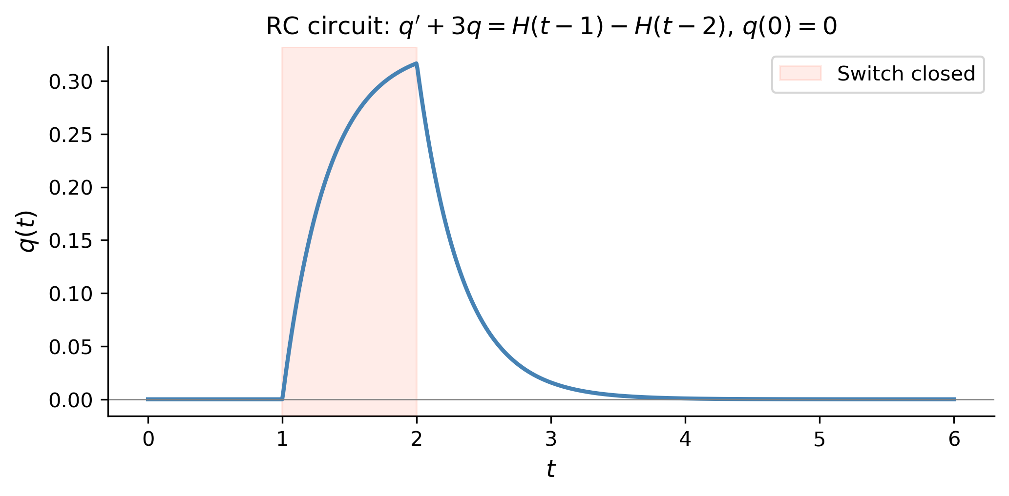
Example. Solve the RC circuit IVP (Logan, Example 3.21): \[ q' + 3q = H(t-1) - H(t-2), \quad q(0) = 0. \]

Step 1. \(sQ(s) + 3Q(s) = \dfrac{1}{s}(e^{-s} - e^{-2s})\).

Step 2. \(Q(s) = \dfrac{1}{s(s+3)}\!\left(e^{-s} - e^{-2s}\right)\).

Step 3. By partial fractions, \(\mathcal{L}^{-1}\!\left[\dfrac{1}{s(s+3)}\right] = \dfrac{1}{3}(1 - e^{-3t})\).

Applying the switching property: \[ \boxed{q(t) = \frac{1}{3}(1-e^{-3(t-1)})H(t-1) - \frac{1}{3}(1-e^{-3(t-2)})H(t-2).} \]

Using SymPy

t, s = sym.symbols('t s', positive=True)
q    = sym.Function('q')

ode_rc = sym.Eq(q(t).diff(t) + 3*q(t),
                sym.Heaviside(t-1) - sym.Heaviside(t-2))
sol_rc = sym.dsolve(ode_rc, q(t), ics={q(0): 0})
display(Math(r'q(t) = ' + sym.latex(sym.simplify(sol_rc.rhs))))

\(\displaystyle q(t) = \frac{\left(- e^{3 t} \theta\left(t - 2\right) + e^{3 t} \theta\left(t - 1\right) + e^{6} \theta\left(t - 2\right) - e^{3} \theta\left(t - 1\right)\right) e^{- 3 t}}{3}\)

Show the code

t_vals = np.linspace(0, 6, 800)

def q_rc(t):
    p1 = np.where(t >= 1, (1/3)*(1 - np.exp(-3*(t-1))), 0)
    p2 = np.where(t >= 2, (1/3)*(1 - np.exp(-3*(t-2))), 0)
    return p1 - p2

fig, ax = plt.subplots(figsize=(7, 3.5))
ax.plot(t_vals, q_rc(t_vals), color='steelblue', lw=2)
ax.axvspan(1, 2, alpha=0.12, color='tomato', label='Switch closed')
ax.axhline(0, color='gray', lw=0.6)
ax.set_xlabel(r'$t$', fontsize=12)
ax.set_ylabel(r'$q(t)$', fontsize=12)
ax.set_title(r"RC circuit: $q' + 3q = H(t-1)-H(t-2)$, $q(0)=0$", fontsize=12)
ax.legend(fontsize=10)
plt.tight_layout()
plt.show()

Figure 3: Charge on the capacitor in the RC circuit (Logan, Example 3.21). The switch closes at \(t=1\), charge builds up, then the switch reopens at \(t=2\) and charge decays.

Tip

Pattern. Express the PWC forcing function in one line with Heaviside functions, using the template: turn on \(g(t)\) at \(t=a\) with \(g(t)H(t-a)\), turn off at \(t=b\) by subtracting \(g(t)H(t-b)\).

B.6 — The Convolution Property

The convolution of \(x(t)\) and \(y(t)\) is \[ (x * y)(t) = \int_0^t x(\tau)\,y(t-\tau)\,d\tau. \] The convolution property (Logan, §3.3) states \[ \mathcal{L}[x * y] = X(s)\,Y(s), \quad\text{equivalently,}\quad \mathcal{L}^{-1}[X(s)Y(s)] = (x*y)(t). \] Convolution is commutative: \(x * y = y * x\).

The convolution is useful for inverting products of transforms when partial fractions would be awkward, and for writing the solution to a DE with an arbitrary forcing function.

By Hand

Example. Invert \(X(s) = \dfrac{3}{s(s^2+9)}\) using convolution (Logan, Example 3.24).

Write \(X(s) = \dfrac{1}{s} \cdot \dfrac{3}{s^2+9}\).

Then \(\mathcal{L}^{-1}[1/s] = 1\) and \(\mathcal{L}^{-1}[3/(s^2+9)] = \sin 3t\).

By convolution: \[ x(t) = 1 * \sin 3t = \int_0^t \sin 3\tau\,d\tau = \frac{1}{3}(1 - \cos 3t). \]

Example. General solution formula (Logan, Example 3.25).

For \(x'' + k^2 x = f(t)\) with initial conditions \(x(0)\), \(x'(0)\), the transform gives \[ X(s) = x(0)\frac{s}{s^2+k^2} + x'(0)\frac{1}{s^2+k^2} + \frac{F(s)}{s^2+k^2}. \] Inverting: \[ x(t) = x(0)\cos kt + \frac{x'(0)}{k}\sin kt + \frac{1}{k}\int_0^t f(\tau)\sin k(t-\tau)\,d\tau. \] The last term is the convolution of \(f\) and \(\tfrac{1}{k}\sin kt\).

Using SymPy

t, tau = sym.symbols('t tau', positive=True)
s      = sym.Symbol('s', positive=True)

# Direct convolution integral: 1 * sin(3t)
conv1 = sym.integrate(sym.sin(3*tau), (tau, 0, t))
display(Math(r'1 * \sin 3t = \int_0^t \sin 3\tau\,d\tau = ' + sym.latex(conv1)))

# Verify via inverse Laplace: L^{-1}[3 / (s(s^2+9))]
X_conv = sym.Integer(3) / (s * (s**2 + 9))
x_conv = sym.inverse_laplace_transform(X_conv, s, t)
display(Math(r'\mathcal{L}^{-1}\!\left[\frac{3}{s(s^2+9)}\right] = '
             + sym.latex(sym.simplify(x_conv))))

# Compute several convolutions from Section 3.3 Exercise 1
pairs = [
    (sym.sin(t),      sym.cos(t),      r'\sin t * \cos t'),
    (sym.exp(-2*t),   sym.exp(-3*t),   r'e^{-2t} * e^{-3t}'),
    (t,               t**2,            r't * t^2'),
]
for f, g, label in pairs:
    result = sym.integrate(
        f.subs(tau, tau) * g.subs(t, t - tau), (tau, 0, t))
    display(Math(label + r' = ' + sym.latex(sym.simplify(result))))

\(\displaystyle 1 * \sin 3t = \int_0^t \sin 3\tau\,d\tau = \frac{1}{3} - \frac{\cos{\left(3 t \right)}}{3}\)

\(\displaystyle \mathcal{L}^{-1}\!\left[\frac{3}{s(s^2+9)}\right] = \frac{1}{3} - \frac{\cos{\left(3 t \right)}}{3}\)

\(\displaystyle \sin t * \cos t = \sin^{2}{\left(t \right)}\)

\(\displaystyle e^{-2t} * e^{-3t} = \frac{\left(e^{3 t} - 1\right) e^{- 5 t}}{3}\)

\(\displaystyle t * t^2 = \frac{t^{4}}{3}\)

Tip

Pattern. When \(X(s) = X_1(s) X_2(s)\), the inverse is the convolution \(x_1 * x_2\). This is especially useful when the product of two recognizable transforms appears, avoiding lengthy partial fractions.

B.7 — Impulsive Sources and the Delta Function

The unit impulse (delta function) \(\delta_a(t)\) at time \(t = a\) is the idealized limit of a rectangular pulse of height \(1/\varepsilon\) and width \(\varepsilon\) as \(\varepsilon \to 0\). It satisfies the sifting property: \[ \int_0^\infty \delta_a(t)\,\phi(t)\,dt = \phi(a). \] Its Laplace transform is \[ \mathcal{L}[\delta_a(t)] = e^{-as}, \qquad \mathcal{L}[\delta_0(t)] = 1. \]

By Hand

Example. Solve \(x'' + x' = \delta_2(t)\), \(x(0) = x'(0) = 0\) (Logan, Example 3.26).

Step 1. \(s^2 X + sX = e^{-2s}\).

Step 2. \(X(s) = \dfrac{e^{-2s}}{s(s+1)}\).

Step 3. \(\mathcal{L}^{-1}[1/(s(s+1))] = 1 - e^{-t}\) (partial fractions).

By the switching property: \[ \boxed{x(t) = H(t-2)(1 - e^{-(t-2)}).} \]

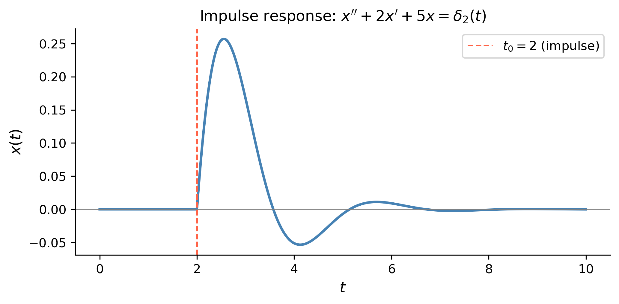
Example. Find the impulse response for \(x'' + 2x' + 5x = \delta_{t_0}(t)\), \(x(0) = x'(0) = 0\) (Logan, Example 3.28).

Transfer function: \(K(s) = 1/(s^2+2s+5) = \tfrac{1}{2} \cdot \dfrac{2}{(s+1)^2+4}\).

Time-domain impulse response: \[ \boxed{x(t) = \tfrac{1}{2}\,H(t-t_0)\,e^{-(t-t_0)}\sin 2(t-t_0).} \]

Using SymPy

t, s = sym.symbols('t s', positive=True)
x    = sym.Function('x')

# Example 3.26: x'' + x' = delta_2(t), x(0)=x'(0)=0
# Build X(s) directly and invert
X_imp = sym.exp(-2*s) / (s*(s+1))
x_imp = sym.inverse_laplace_transform(X_imp, s, t)
display(Math(r'\text{Ex 3.26: }x(t) = ' + sym.latex(sym.simplify(x_imp))))

# Transfer function for x'' + 2x' + 5x = delta_{t0}(t)
t0 = sym.Symbol('t_0', positive=True)
K_s = 1 / (s**2 + 2*s + 5)
display(Math(r'K(s) = ' + sym.latex(sym.simplify(K_s))
             + r' = \frac{1}{2}\cdot\frac{2}{(s+1)^2+4}'))

# Impulse response with t0 = 2
X_t0 = K_s * sym.exp(-2*s)
x_t0 = sym.inverse_laplace_transform(X_t0, s, t)
display(Math(r'x(t)\text{ (}t_0=2\text{)} = '
             + sym.latex(sym.simplify(x_t0))))

\(\displaystyle \text{Ex 3.26: }x(t) = \left(e^{t} - e^{2}\right) e^{- t} \theta\left(t - 2\right)\)

\(\displaystyle K(s) = \frac{1}{s^{2} + 2 s + 5} = \frac{1}{2}\cdot\frac{2}{(s+1)^2+4}\)

\(\displaystyle x(t)\text{ (}t_0=2\text{)} = \frac{e^{2 - t} \sin{\left(2 t - 4 \right)} \theta\left(t - 2\right)}{2}\)

Show the code

t_vals = np.linspace(0, 10, 800)
t0_val = 2.0

x_resp = np.where(
    t_vals >= t0_val,
    0.5 * np.exp(-(t_vals - t0_val)) * np.sin(2*(t_vals - t0_val)),
    0.0
)

fig, ax = plt.subplots(figsize=(7, 3.5))
ax.plot(t_vals, x_resp, color='steelblue', lw=2)
ax.axvline(t0_val, color='tomato', ls='--', lw=1.2,
           label=r'$t_0 = 2$ (impulse)')
ax.axhline(0, color='gray', lw=0.6)
ax.set_xlabel(r'$t$', fontsize=12)
ax.set_ylabel(r'$x(t)$', fontsize=12)
ax.set_title(r"Impulse response: $x''+2x'+5x=\delta_2(t)$", fontsize=12)
ax.legend(fontsize=10)
plt.tight_layout()
plt.show()

Figure 4: Impulse response of \(x''+2x'+5x=\delta_{t_0}(t)\) for \(t_0=2\) (Logan, Example 3.28). The system is at rest until \(t=2\), then undergoes a decaying oscillation.

Tip

Pattern. An impulsive source \(\delta_a(t)\) contributes \(e^{-as}\) to the right-hand side of the transformed equation. After solving for \(X(s)\), invert using the switching property; the result is zero for \(t < a\) and a decaying (or oscillating) response for \(t > a\).

B.8 — Transfer Functions and Input–Output Systems

For the linear system with zero initial conditions \[ ax'' + bx' + cx = f(t), \quad x(0) = x'(0) = 0, \] the forced response in the transform domain is \[ X(s) = K(s)\,F(s), \] where \[ K(s) = \frac{1}{as^2 + bs + c} \] is the transfer function. In the time domain, the forced response is the convolution \(x(t) = k(t) * f(t)\), where \(k(t) = \mathcal{L}^{-1}[K(s)]\).

The transfer function fully characterizes the system’s response to any input, without needing to solve the DE from scratch each time.

By Hand

Example. Find the transfer function and impulse response for \(x'' + 2x' + 5x = f(t)\) (Logan, §3.4).

\[ K(s) = \frac{1}{s^2+2s+5} = \frac{1}{2}\cdot\frac{2}{(s+1)^2+4}. \]

\[ k(t) = \mathcal{L}^{-1}[K(s)] = \frac{1}{2}\,e^{-t}\sin 2t. \]

For any input \(f(t)\), the forced response is \[ x(t) = \frac{1}{2}\int_0^t e^{-(t-\tau)}\sin 2(t-\tau)\,f(\tau)\,d\tau. \]

Using Python — Comparing Step and Impulse Responses

Show the code

def system_rhs(t, state, f_func):
    x_val, xdot = state
    return [xdot, f_func(t) - 2*xdot - 5*x_val]

t_span = (0, 10)
t_eval = np.linspace(*t_span, 800)

inputs = {
    r'Impulse $\delta_\varepsilon(t)$, $\varepsilon=0.05$':
        lambda t: (1/0.05) if (0 <= t < 0.05) else 0,
    r'Unit step $H(t)$':
        lambda t: 1.0,
    r'Sinusoid $\sin 2t$':
        lambda t: np.sin(2*t),
}
colors = ['steelblue', 'tomato', 'seagreen']

fig, axes = plt.subplots(1, 3, figsize=(12, 3.5), sharey=False)

for ax, (label, f_in), color in zip(axes, inputs.items(), colors):
    sol = solve_ivp(system_rhs, t_span, [0, 0],
                    args=(f_in,), t_eval=t_eval,
                    max_step=0.01, rtol=1e-8)
    ax.plot(sol.t, sol.y[0], color=color, lw=2)
    ax.axhline(0, color='gray', lw=0.5)
    ax.set_xlabel(r'$t$', fontsize=11)
    ax.set_ylabel(r'$x(t)$', fontsize=11)
    ax.set_title(label, fontsize=10)

plt.suptitle(r"Transfer function demo: $x''+2x'+5x=f(t)$", fontsize=12)
plt.tight_layout()
plt.show()

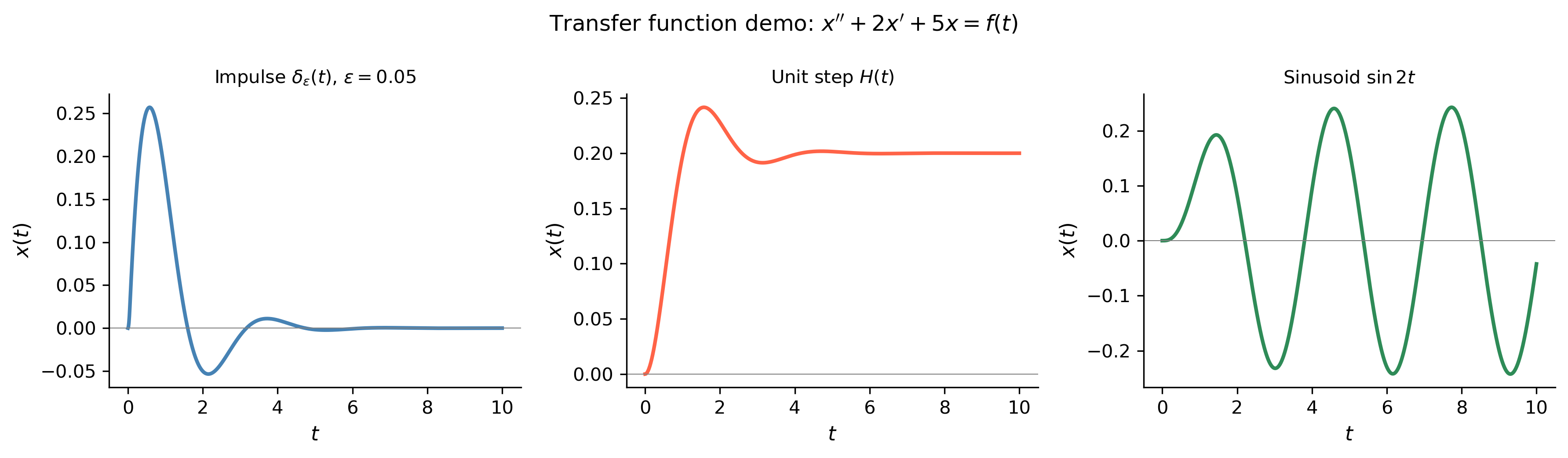
Figure 5: Responses of \(x''+2x'+5x=f(t)\), \(x(0)=x'(0)=0\) to three canonical inputs: an impulse \(\delta_0(t)\), a unit step \(H(t)\), and a sinusoidal input \(\sin(2t)\). All solved numerically with `scipy.integrate.solve_ivp`.

Tip

Pattern. The transfer function \(K(s)\) encodes everything about the system. The impulse response \(k(t) = \mathcal{L}^{-1}[K(s)]\) determines the response to any input via \(x(t) = k * f\). In practice, solve_ivp gives the numerical response for arbitrary \(f(t)\) without needing to compute the convolution integral analytically.

B.9 — Selected Review Exercises

This section works through a selection of exercises from Logan Chapter 3, following the same by-hand and Python structure used throughout.

Exercise 3.1.8 — Computing Transforms

Problem. Find the Laplace transform of each function.

\(6 + 5e^{-2t} + te^{3t}\) (b) \(\cos 5t\) (c) \(3e^{-t}\cosh t\) (f) \(H(t-\pi)\cos(t-\pi)\)

By Hand.

By linearity and the table: \[ \mathcal{L}[6 + 5e^{-2t} + te^{3t}] = \frac{6}{s} + \frac{5}{s+2} + \frac{1}{(s-3)^2}. \]
\(\mathcal{L}[\cos 5t] = \dfrac{s}{s^2+25}\).
\(\cosh t = (e^t + e^{-t})/2\), so \(e^{-t}\cosh t = (1 + e^{-2t})/2\). \[ \mathcal{L}[3e^{-t}\cosh t] = \frac{3}{2}\!\left(\frac{1}{s} + \frac{1}{s+2}\right) = \frac{3(s+1)}{s(s+2)}. \] Alternatively by the shift property with \(\mathcal{L}[\cosh t] = s/(s^2-1)\): \(\mathcal{L}[e^{-t}\cosh t] = (s+1)/((s+1)^2-1) = (s+1)/(s^2+2s)\).
Switching property with \(a = \pi\), \(f(t) = \cos t\): \[ \mathcal{L}[H(t-\pi)\cos(t-\pi)] = e^{-\pi s}\cdot\frac{s}{s^2+1}. \]

t, s = sym.symbols('t s', positive=True)

for label, f in [
    (r'6 + 5e^{-2t} + te^{3t}',
     6 + 5*sym.exp(-2*t) + t*sym.exp(3*t)),
    (r'\cos 5t',
     sym.cos(5*t)),
    (r'3e^{-t}\cosh t',
     3*sym.exp(-t)*sym.cosh(t)),
    (r'H(t-\pi)\cos(t-\pi)',
     sym.Heaviside(t - sym.pi)*sym.cos(t - sym.pi)),
]:
    F, *_ = sym.laplace_transform(f, t, s, noconds=False)
    display(Math(r'\mathcal{L}\!\left[' + label + r'\right] = '
                 + sym.latex(sym.simplify(F))))

\(\displaystyle \mathcal{L}\!\left[6 + 5e^{-2t} + te^{3t}\right] = \frac{5}{s + 2} + \frac{1}{\left(s - 3\right)^{2}} + \frac{6}{s}\)

\(\displaystyle \mathcal{L}\!\left[\cos 5t\right] = \frac{s}{s^{2} + 25}\)

\(\displaystyle \mathcal{L}\!\left[3e^{-t}\cosh t\right] = \frac{3 \left(s + 1\right)}{s \left(s + 2\right)}\)

\(\displaystyle \mathcal{L}\!\left[H(t-\pi)\cos(t-\pi)\right] = \frac{s e^{- \pi s}}{s^{2} + 1}\)

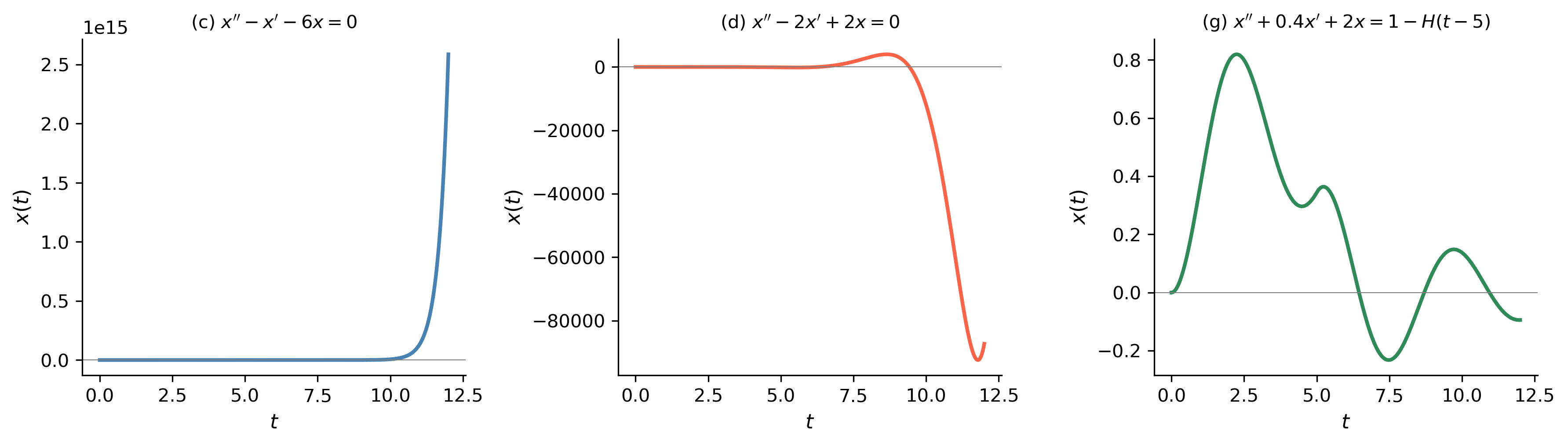
Exercise 3.2.6 — Solving IVPs by Laplace Transforms

Problem. Solve selected IVPs from Logan §3.2 Exercise 6.

\(x'' - x' - 6x = 0\), \(x(0) = 2\), \(x'(0) = -1\).
\(x'' - 2x' + 2x = 0\), \(x(0) = 0\), \(x'(0) = 1\).
\(x'' + 0.4x' + 2x = 1 - H(t-5)\), \(x(0) = x'(0) = 0\).

By Hand — (c).

Transform: \((s^2 - s - 6)X = 2s - 1 - 2 = 2s - 3\). \[ X(s) = \frac{2s-3}{(s-3)(s+2)}. \] Partial fractions: \(A/(s-3) + B/(s+2)\) with \(A = 3/5\), \(B = 7/5\). \[ x(t) = \frac{3}{5}e^{3t} + \frac{7}{5}e^{-2t}. \]

By Hand — (d).

Characteristic roots: \(\lambda = 1 \pm i\). Transform: \((s^2 - 2s + 2)X = 1\). \(X(s) = 1/((s-1)^2+1)\). \[ x(t) = e^t \sin t. \]

t, s = sym.symbols('t s', positive=True)
x    = sym.Function('x')

ivps = [
    (sym.Eq(x(t).diff(t,2) - x(t).diff(t) - 6*x(t), 0),
     {x(0): 2, x(t).diff(t).subs(t,0): -1},
     r'\text{(c)}'),
    (sym.Eq(x(t).diff(t,2) - 2*x(t).diff(t) + 2*x(t), 0),
     {x(0): 0, x(t).diff(t).subs(t,0): 1},
     r'\text{(d)}'),
    (sym.Eq(x(t).diff(t,2) + sym.Rational(2,5)*x(t).diff(t) + 2*x(t),
            1 - sym.Heaviside(t-5)),
     {x(0): 0, x(t).diff(t).subs(t,0): 0},
     r'\text{(g)}'),
]

for ode, ics, label in ivps:
    sol = sym.dsolve(ode, x(t), ics=ics)
    display(Math(label + r': x(t) = ' + sym.latex(sym.simplify(sol.rhs))))

\(\displaystyle \text{(c)}: x(t) = \frac{\left(3 e^{5 t} + 7\right) e^{- 2 t}}{5}\)

\(\displaystyle \text{(d)}: x(t) = e^{t} \sin{\left(t \right)}\)

\(\displaystyle \text{(g)}: x(t) = \frac{\left(7 \left(1 - \theta\left(t - 5\right)\right) e^{\frac{t}{5}} - \sin{\left(\frac{7 t}{5} \right)} + e \sin{\left(\frac{7 t}{5} - 7 \right)} \theta\left(t - 5\right) - 7 \cos{\left(\frac{7 t}{5} \right)} + 7 e \cos{\left(\frac{7 t}{5} - 7 \right)} \theta\left(t - 5\right)\right) e^{- \frac{t}{5}}}{14}\)

Show the code

t_vals = np.linspace(0, 12, 800)

def rhs_c(t, y): return [y[1], y[1] + 6*y[0]]
def rhs_d(t, y): return [y[1], 2*y[1] - 2*y[0]]
def rhs_g(t, y):
    f = 1.0 if t < 5 else 0.0
    return [y[1], f - 0.4*y[1] - 2*y[0]]

problems = [
    (rhs_c, [2, -1],  r"(c) $x''-x'-6x=0$",          'steelblue'),
    (rhs_d, [0,  1],  r"(d) $x''-2x'+2x=0$",          'tomato'),
    (rhs_g, [0,  0],  r"(g) $x''+0.4x'+2x=1-H(t-5)$", 'seagreen'),
]

fig, axes = plt.subplots(1, 3, figsize=(12, 3.5))
for ax, (rhs, y0, title, color) in zip(axes, problems):
    sol = solve_ivp(rhs, (0, 12), y0, t_eval=t_vals, rtol=1e-9)
    ax.plot(sol.t, sol.y[0], color=color, lw=2)
    ax.axhline(0, color='gray', lw=0.5)
    ax.set_xlabel(r'$t$', fontsize=11)
    ax.set_ylabel(r'$x(t)$', fontsize=11)
    ax.set_title(title, fontsize=10)
plt.tight_layout()
plt.show()

Figure 6: Solutions to three IVPs from Logan §3.2, Exercise 6. Panel (g) shows the effect of a step input that switches off at \(t=5\): the oscillation continues with the homogeneous (free) response thereafter.

Exercise 3.3.1 — Convolution Integrals

Problem. Compute the convolutions: (a) \(\sin t * \cos t\), (b) \(e^{-2t}*e^{-3t}\), (c) \(t * t^2\), (d) \(t * e^t\).

By Hand — (b). \(e^{-2t}*e^{-3t} = \int_0^t e^{-2\tau}e^{-3(t-\tau)}\,d\tau = e^{-3t}\int_0^t e^{\tau}\,d\tau = e^{-3t}(e^t - 1) = e^{-2t} - e^{-3t}\).

Verification via Laplace: \(\mathcal{L}^{-1}\!\left[\dfrac{1}{(s+2)(s+3)}\right] = e^{-2t} - e^{-3t}\) ✓.

t, tau = sym.symbols('t tau', nonnegative=True)
s      = sym.Symbol('s', positive=True)

convolutions = [
    (sym.sin(tau),    sym.cos(t - tau),   r'\sin t * \cos t'),
    (sym.exp(-2*tau), sym.exp(-3*(t-tau)),r'e^{-2t}*e^{-3t}'),
    (tau,             (t-tau)**2,          r't * t^2'),
    (tau,             sym.exp(t - tau),    r't * e^t'),
]

for f, g, label in convolutions:
    result = sym.simplify(sym.integrate(f * g, (tau, 0, t)))
    display(Math(label + r' = ' + sym.latex(result)))

\(\displaystyle \sin t * \cos t = \frac{t \sin{\left(t \right)}}{2}\)

\(\displaystyle e^{-2t}*e^{-3t} = \left(e^{t} - 1\right) e^{- 3 t}\)

\(\displaystyle t * t^2 = \frac{t^{4}}{12}\)

\(\displaystyle t * e^t = - t + e^{t} - 1\)

Exercise 3.4 — Impulse Problems with Visualization

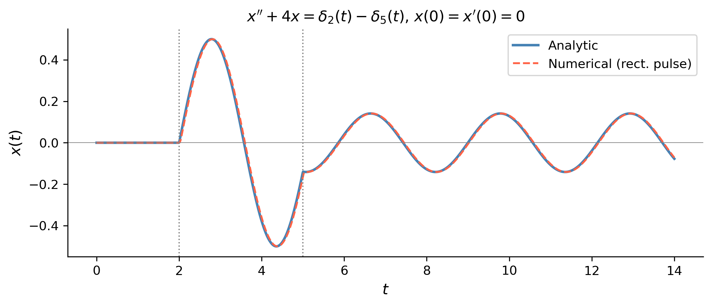
Problem. Solve \(x'' + 4x = \delta_2(t) - \delta_5(t)\), \(x(0) = x'(0) = 0\) (Logan, §3.4 Exercise 6).

By Hand.

Transform: \((s^2+4)X = e^{-2s} - e^{-5s}\).

\(X(s) = \dfrac{e^{-2s} - e^{-5s}}{s^2+4} = \dfrac{1}{2}\cdot\dfrac{2}{s^2+4}(e^{-2s} - e^{-5s})\).

Since \(\mathcal{L}^{-1}[2/(s^2+4)] = \sin 2t\), by the switching property: \[ \boxed{x(t) = \frac{1}{2}H(t-2)\sin 2(t-2) - \frac{1}{2}H(t-5)\sin 2(t-5).} \]

Show the code

t_vals = np.linspace(0, 14, 1400)

# Analytic solution
def x_analytic(t):
    p1 = np.where(t >= 2, 0.5*np.sin(2*(t-2)), 0.0)
    p2 = np.where(t >= 5, 0.5*np.sin(2*(t-5)), 0.0)
    return p1 - p2

# Numerical: approximate delta with narrow rectangle of width eps
eps = 0.05
def rhs_double(t, y):
    d2 = (1/eps) if (2 <= t < 2+eps) else 0.0
    d5 = (1/eps) if (5 <= t < 5+eps) else 0.0
    return [y[1], (d2 - d5) - 4*y[0]]

sol_num = solve_ivp(rhs_double, (0, 14), [0, 0],
                    t_eval=t_vals, max_step=0.005, rtol=1e-9)

fig, ax = plt.subplots(figsize=(8, 3.5))
ax.plot(t_vals, x_analytic(t_vals), color='steelblue', lw=2,
        label='Analytic')
ax.plot(sol_num.t, sol_num.y[0], color='tomato', lw=1.5,
        ls='--', label='Numerical (rect. pulse)')
ax.axvline(2, color='gray', ls=':', lw=1)
ax.axvline(5, color='gray', ls=':', lw=1)
ax.axhline(0, color='gray', lw=0.5)
ax.set_xlabel(r'$t$', fontsize=12)
ax.set_ylabel(r'$x(t)$', fontsize=12)
ax.set_title(r"$x''+4x = \delta_2(t)-\delta_5(t)$, $x(0)=x'(0)=0$",
             fontsize=12)
ax.legend(fontsize=10)
plt.tight_layout()
plt.show()

Figure 7: Response of \(x''+4x = \delta_2(t)-\delta_5(t)\), \(x(0)=x'(0)=0\) (Logan §3.4, Ex. 6). The first impulse at \(t=2\) starts oscillation; the second at \(t=5\) modifies it. Compare the analytic solution (solid) with `solve_ivp` using a narrow rectangular pulse (dashed).

B.10 — Summary: The Laplace Transform Toolkit

The table below (Logan, Table 3.1) collects the essential transform pairs. SymPy can verify every entry.

Show the code — verify Table 3.1 entries

t, s, k, a, n = sym.symbols('t s k a n', positive=True)

entries = [
    (r'e^{at}',           sym.exp(a*t)),
    (r't^n',              t**3),            # n=3 as example
    (r'\sin kt',          sym.sin(k*t)),
    (r'\cos kt',          sym.cos(k*t)),
    (r'\sinh kt',         sym.sinh(k*t)),
    (r'\cosh kt',         sym.cosh(k*t)),
    (r'e^{at}\sin kt',    sym.exp(a*t)*sym.sin(k*t)),
    (r'e^{at}\cos kt',    sym.exp(a*t)*sym.cos(k*t)),
    (r'H(t-a)',           sym.Heaviside(t-a)),
    (r'\delta_a(t)',       sym.DiracDelta(t-a)),
]

print(f"{'x(t)':<25}  X(s)")
print("-" * 60)
for label, f in entries:
    F, *_ = sym.laplace_transform(f, t, s, noconds=False)
    print(f"  {label:<23}  {sym.simplify(F)}")

x(t)                       X(s)
------------------------------------------------------------
  e^{at}                   1/(-a + s)
  t^n                      6/s**4
  \sin kt                  k/(k**2 + s**2)
  \cos kt                  s/(k**2 + s**2)
  \sinh kt                 k/(-k**2 + s**2)
  \cosh kt                 s/(-k**2 + s**2)
  e^{at}\sin kt            k/(k**2 + (a - s)**2)
  e^{at}\cos kt            (-a + s)/(k**2 + (a - s)**2)
  H(t-a)                   exp(-a*s)/s
  \delta_a(t)              exp(-a*s)

Note

The three-step Laplace method — at a glance.

Transform the IVP: replace \(x'\) by \(sX - x(0)\) and \(x''\) by \(s^2X - sx(0) - x'(0)\); use linearity.
Solve the resulting algebraic equation for \(X(s)\).
Invert \(X(s)\) using the table, partial fractions, completing the square, the switching property (\(e^{-as}\) signals a time delay), and convolution.

References

Logan, J David. 2015. A First Course in Differential Equations, Third Edition.

Expand for Session Info

import sys, importlib
print("Python version:", sys.version)
for name in ['numpy', 'sympy', 'scipy', 'matplotlib']:
    mod = importlib.import_module(name)
    print(f"{name}=={mod.__version__}")

Python version: 3.14.4 | packaged by conda-forge | (main, Apr  8 2026, 02:33:53) [Clang 20.1.8 ]
numpy==2.4.3
sympy==1.14.0
scipy==1.17.1
matplotlib==3.10.8

Reuse

CC BY-NC-SA 4.0