Bernoulli Equations

Show the code
import numpy as np
import sympy as sym
import matplotlib as mpl
import matplotlib.pyplot as plt
from scipy.integrate import solve_ivp
from IPython.display import Math, display
mpl.rcParams['figure.dpi'] = 150
mpl.rcParams['axes.spines.top'] = False
mpl.rcParams['axes.spines.right'] = False

This section discusses Bernoulli equations, a class of nonlinear first-order ODEs that can be transformed into a linear equation by a clever substitution. They arise naturally in population dynamics, fluid mechanics, and mathematical biology, and provide an important example of how a nonlinear ODE can sometimes be solved exactly by reducing it to a linear one. The material here supplements Exercises 14–15 in Section 1.4.1 of Logan (2015).


Historical Background

The Bernoulli equation bears the name of the Swiss mathematician Jacob Bernoulli (1655–1705), who posed the problem in 1695. It was solved independently and almost simultaneously by his younger brother Johann Bernoulli (1667–1748) and by Gottfried Wilhelm Leibniz (1646–1716).

Leibniz’s approach — a substitution that reduces the nonlinear equation to a linear one — is exactly what we use today. The episode is historically notable because it was one of the first demonstrations that a class of nonlinear ODEs could be solved in closed form by a systematic technique, not just by inspection.

The two Bernoulli brothers were towering figures in early calculus. Jacob contributed the law of large numbers in probability and the study of the catenary (the curve of a hanging chain); Johann taught Guillaume de l’Hôpital and later became the mentor of Leonhard Euler. The family produced no fewer than eight notable mathematicians across three generations.

Note

The term “Bernoulli equation” can refer to two entirely different results: this ODE, and also the Bernoulli principle in fluid dynamics (pressure–velocity trade-off in a flowing fluid), named after Jacob’s nephew Daniel Bernoulli (1700–1782). They are unrelated beyond the family name.


Definition

A Bernoulli equation is a first-order ODE of the form \[ x' = a(t)\,x + g(t)\,x^n, \tag{B} \] where \(a(t)\) and \(g(t)\) are continuous functions of \(t\) and \(n\) is a real constant.

Special cases.

Value of \(n\) Character Reduces to
\(n = 0\) Linear \(x' = a(t)x + g(t)\) directly
\(n = 1\) Linear (separable) \(x' = [a(t)+g(t)]x\)
\(n \neq 0, 1\) Nonlinear Linear after substitution

The interesting and non-trivial case is \(n \neq 0, 1\), which is genuinely nonlinear.


The Leibniz Substitution

The key observation is that the substitution \[ y = x^{1-n} \] transforms (B) into a linear ODE for \(y(t)\).

Derivation. Assume \(x \neq 0\) and differentiate \(y = x^{1-n}\): \[ y' = (1-n)\,x^{-n}\,x'. \] Substituting \(x' = a(t)x + g(t)x^n\) from (B): \[ y' = (1-n)\,x^{-n}\bigl[a(t)x + g(t)x^n\bigr] = (1-n)\,a(t)\,x^{1-n} + (1-n)\,g(t). \] Since \(x^{1-n} = y\) this becomes: \[ \boxed{y' - (1-n)\,a(t)\,y = (1-n)\,g(t).} \tag{L} \] This is a first-order linear ODE in \(y\), solvable by the integrating factor method. Once \(y(t)\) is found, the solution to (B) is recovered by \[ x(t) = y(t)^{1/(1-n)}. \]

ImportantSummary of the Method
  1. Identify \(n\), \(a(t)\), \(g(t)\) in \(x' = a(t)x + g(t)x^n\).
  2. Substitute \(y = x^{1-n}\) to obtain the linear ODE \(y' - (1-n)a(t)y = (1-n)g(t)\).
  3. Solve for \(y(t)\) using an integrating factor.
  4. Recover \(x(t) = y^{1/(1-n)}\).
  5. Append any solution \(x \equiv 0\) that was lost by assuming \(x \neq 0\).
Tip

The trivial solution. Dividing by \(x^n\) in step 2 requires \(x \neq 0\). But \(x(t) \equiv 0\) always satisfies (B) (substitute and check). The general family from step 3 may or may not include it as a limiting case; it should always be stated separately.


Worked Examples

Example 1 — \(x' = x + x^2 e^t\)

Here \(n = 2\), \(a(t) = 1\), \(g(t) = e^t\).

Step 1. Substitute \(y = x^{1-2} = x^{-1}\).

Step 2. The linear ODE (L) is: \[ y' - (1-2)(1)\,y = (1-2)\,e^t \quad\Longrightarrow\quad y' + y = -e^t. \]

Step 3. Integrating factor: \(\mu = e^t\). \[ (ye^t)' = -e^{2t} \quad\Longrightarrow\quad ye^t = -\tfrac{1}{2}e^{2t} + C \quad\Longrightarrow\quad y = -\tfrac{1}{2}e^t + Ce^{-t}. \]

Step 4. \(x = y^{-1}\): \[ \boxed{x(t) = \frac{1}{Ce^{-t} - \tfrac{1}{2}e^t} = \frac{2e^t}{2C - e^{2t}}.} \]

Also \(x(t) \equiv 0\) is a solution.

Note

Finite-time blow-up. The denominator \(2C - e^{2t}\) vanishes at \(t^* = \tfrac{1}{2}\ln(2C)\). This means solutions blow up to \(\pm\infty\) in finite time — a hallmark of nonlinear ODEs that linear equations never exhibit. For an initial condition \(x(0) = x_0 > 0\), we get \(C = 1/x_0 + 1/2\) and the blow-up time is \(t^* = \tfrac{1}{2}\ln(2/x_0 + 1)\). Smaller \(x_0\) gives later blow-up; larger \(x_0\) blows up sooner.

Show the code
def x_ex1_closed(t, x0):
    C = 1.0/x0 + 0.5
    denom = 2*C - np.exp(2*t)
    return np.where(denom > 0.01, 2*np.exp(t)/denom, np.nan)

f_b = lambda t, x: [x[0]*(1 + x[0]*np.exp(t))]

fig, ax = plt.subplots(figsize=(8, 5))
colors = plt.cm.viridis(np.linspace(0.15, 0.85, 4))
x0_vals = [0.2, 0.4, 0.6, 0.8]

for x0, color in zip(x0_vals, colors):
    C = 1/x0 + 0.5
    t_blow = 0.5*np.log(2*C)
    t_safe = np.linspace(0, t_blow - 0.05, 400)

    # Closed-form
    x_clo = 2*np.exp(t_safe)/(2*C - np.exp(2*t_safe))
    ax.plot(t_safe, x_clo, color=color, lw=2.5, label=f'$x_0={x0}$, $t^*={t_blow:.2f}$')

    # Numerical check (dots)
    sol = solve_ivp(f_b, (0, t_blow-0.08), [x0], dense_output=True, max_step=0.005)
    t_dots = np.linspace(0, t_blow-0.12, 12)
    ax.plot(t_dots, sol.sol(t_dots)[0], 'o', color=color, markersize=5)

    # Blow-up marker
    ax.axvline(t_blow, color=color, linestyle=':', lw=1.2, alpha=0.7)

ax.set_ylim(0, 20)
ax.set_xlabel('$t$')
ax.set_ylabel('$x(t)$')
ax.set_title(r"$x' = x + x^2 e^t$: finite-time blow-up")
ax.legend(fontsize=9)
plt.tight_layout()
plt.show()
Figure 1: Solutions of \(x' = x + x^2 e^t\) from several initial conditions \(x_0 > 0\). Each solution blows up at \(t^* = \frac{1}{2}\ln(2/x_0+1)\) (marked with a vertical dashed line). The closed-form solution (solid) agrees perfectly with the numerical ODE solve (dots).

Example 2 — \(x' = ax + bx^3\) (Constant Coefficients)

Here \(n = 3\), \(a(t) = a\) (constant), \(g(t) = b\) (constant). This equation arises in nonlinear oscillation theory, optics (Kerr effect), and population models.

Step 1. Substitute \(y = x^{1-3} = x^{-2}\).

Step 2. The linear ODE: \[ y' - (1-3)a\,y = (1-3)b \quad\Longrightarrow\quad y' + 2ay = -2b. \]

Step 3. Integrating factor: \(\mu = e^{2at}\). \[ (ye^{2at})' = -2b\,e^{2at} \quad\Longrightarrow\quad y = -\frac{b}{a} + \left(y_0 + \frac{b}{a}\right)e^{-2at}, \] where \(y_0 = x_0^{-2} = 1/x(0)^2\).

Step 4. \(x = y^{-1/2}\): \[ \boxed{x(t) = \frac{1}{\displaystyle\sqrt{-\frac{b}{a} + \!\left(\frac{1}{x_0^2}+\frac{b}{a}\right)e^{-2at}}}.} \]

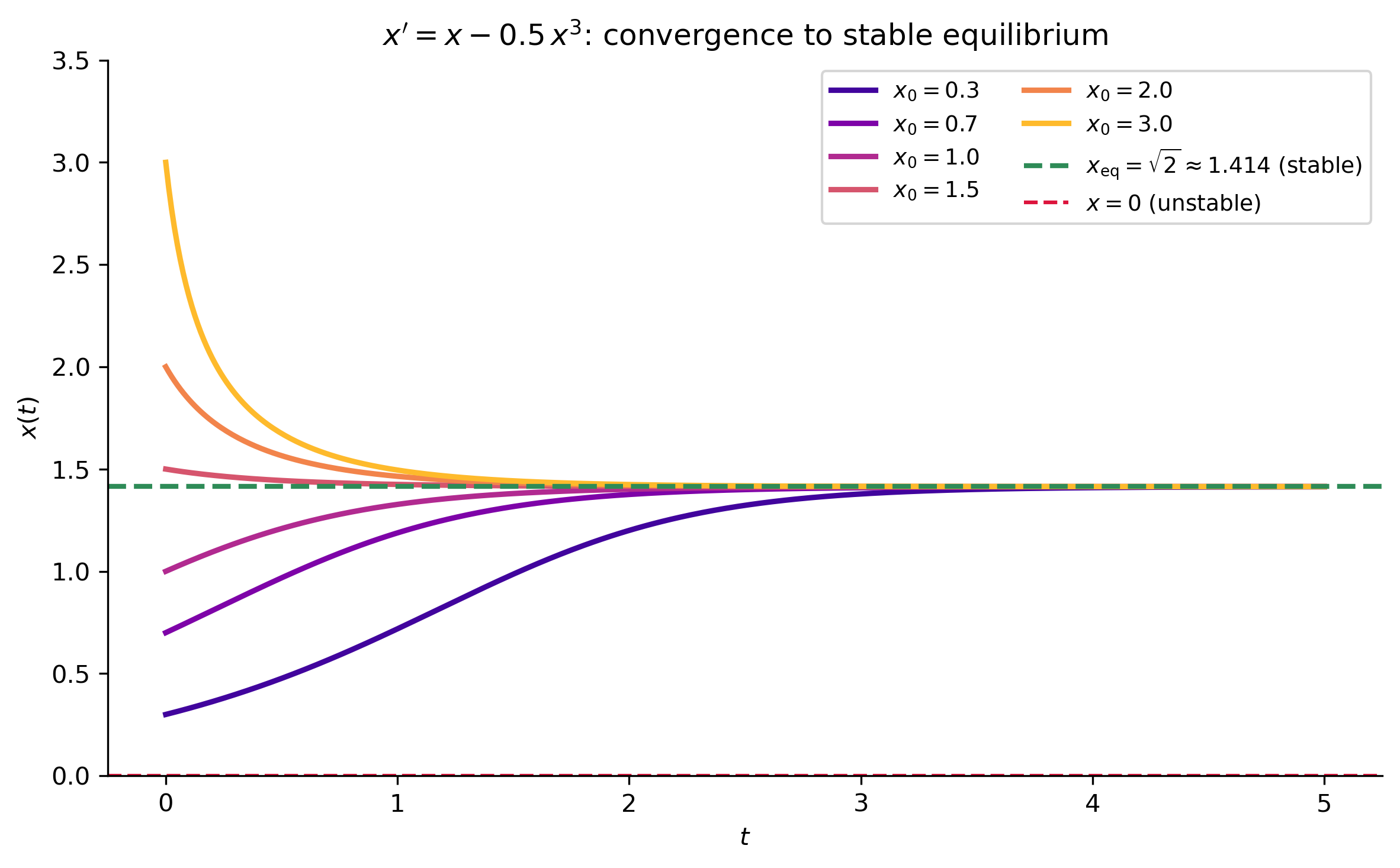
Equilibria (setting \(x' = 0\) for non-zero \(x\)): \(ax + bx^3 = x(a+bx^2) = 0\), giving \(x = 0\) and \(x = \pm\sqrt{-a/b}\) (real only when \(a/b < 0\)).

When \(a > 0\) and \(b < 0\) (so \(-b/a > 0\)), there is a non-zero equilibrium \(x_{\text{eq}} = \sqrt{-a/b}\) that acts as an attractor for \(x > 0\).

Show the code
a_val, b_val = 1.0, -0.5
x_eq = np.sqrt(-a_val / b_val)   # = sqrt(2)

def x_ex2_closed(t, x0, a, b):
    y0 = 1.0 / x0**2
    y_t = -b/a + (y0 + b/a)*np.exp(-2*a*t)
    return 1.0 / np.sqrt(np.abs(y_t)) * np.sign(x0)

f_e = lambda t, x: [a_val*x[0] + b_val*x[0]**3]

fig, ax = plt.subplots(figsize=(8, 5))
colors = plt.cm.plasma(np.linspace(0.1, 0.85, 6))
x0_vals = [0.3, 0.7, 1.0, 1.5, 2.0, 3.0]
t_plot = np.linspace(0, 5, 400)

for x0, color in zip(x0_vals, colors):
    x_clo = x_ex2_closed(t_plot, x0, a_val, b_val)
    ax.plot(t_plot, x_clo, color=color, lw=2.2, label=f'$x_0={x0}$')

ax.axhline(x_eq, color='seagreen', ls='--', lw=2, label=f'$x_{{\\rm eq}}=\\sqrt{{2}}\\approx{x_eq:.3f}$ (stable)')
ax.axhline(0,    color='crimson',  ls='--', lw=1.5, label='$x=0$ (unstable)')
ax.set_xlabel('$t$')
ax.set_ylabel('$x(t)$')
ax.set_title(r"$x' = x - 0.5\,x^3$: convergence to stable equilibrium")
ax.set_ylim(0, 3.5)
ax.legend(fontsize=9, ncol=2)
plt.tight_layout()
plt.show()
Figure 2: Solutions of \(x' = x - 0.5x^3\) (\(a=1\), \(b=-0.5\)) from several initial conditions. The non-zero equilibrium \(x_{\rm eq} = \sqrt{2} \approx 1.414\) (dashed green) is stable: all solutions with \(x_0>0\) converge to it. The trivial equilibrium \(x=0\) (dashed red) is unstable.

Example 3 — The Logistic Equation as a Bernoulli Equation

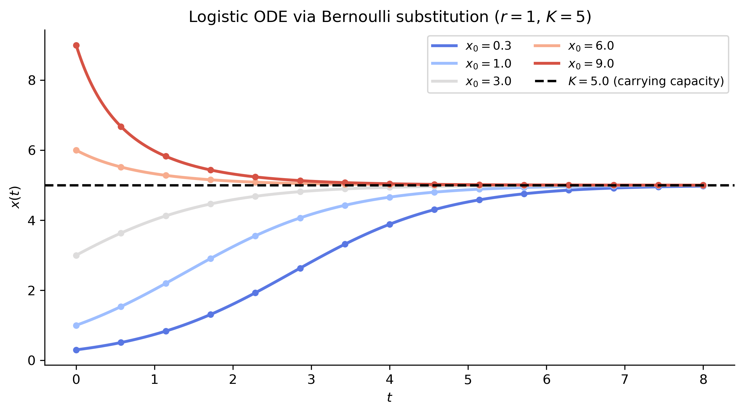
The logistic equation \[ x' = rx\!\left(1 - \frac{x}{K}\right) = rx - \frac{r}{K}x^2 \] is a Bernoulli equation with \(n = 2\), \(a(t) = r\), \(g(t) = -r/K\).

Substitution \(y = x^{-1}\) gives: \[ y' + ry = \frac{r}{K}, \] a linear ODE with constant coefficients. The integrating factor is \(e^{rt}\): \[ (ye^{rt})' = \frac{r}{K}e^{rt} \quad\Longrightarrow\quad y = \frac{1}{K} + Ce^{-rt}. \] Applying \(y(0) = 1/x_0\): \[ C = \frac{1}{x_0} - \frac{1}{K} = \frac{K - x_0}{Kx_0}, \] and recovering \(x = 1/y\): \[ x(t) = \frac{1}{1/K + Ce^{-rt}} = \frac{K}{1 + (K/x_0 - 1)e^{-rt}}, \] which is exactly the familiar logistic solution — now derived via the Bernoulli substitution as an alternative to partial fractions.

Show the code
r_val, K_val = 1.0, 5.0

def logistic_closed(t, x0, r, K):
    return K / (1 + (K/x0 - 1)*np.exp(-r*t))

f_log = lambda t, x: [r_val*x[0]*(1 - x[0]/K_val)]

fig, ax = plt.subplots(figsize=(8, 4.5))
colors = plt.cm.coolwarm(np.linspace(0.1, 0.9, 5))
x0_vals = [0.3, 1.0, 3.0, 6.0, 9.0]
t_plot  = np.linspace(0, 8, 400)

for x0, color in zip(x0_vals, colors):
    x_clo = logistic_closed(t_plot, x0, r_val, K_val)
    ax.plot(t_plot, x_clo, color=color, lw=2.2, label=f'$x_0={x0}$')
    sol = solve_ivp(f_log, (0, 8), [x0], dense_output=True, max_step=0.05)
    t_dots = np.linspace(0, 8, 15)
    ax.plot(t_dots, sol.sol(t_dots)[0], 'o', color=color, markersize=4)

ax.axhline(K_val, color='black', ls='--', lw=1.8, label=f'$K={K_val}$ (carrying capacity)')
ax.set_xlabel('$t$')
ax.set_ylabel('$x(t)$')
ax.set_title(r"Logistic ODE via Bernoulli substitution ($r=1$, $K=5$)")
ax.legend(fontsize=9, ncol=2)
plt.tight_layout()
plt.show()
Figure 3: Logistic growth (\(r=1\), \(K=5\)) solved via the Bernoulli substitution. The closed-form solution (solid) is compared to a direct numerical solve (dots) for four initial conditions. All solutions converge to the carrying capacity \(K=5\) (dashed).

Example 4 — SymPy: Solving Bernoulli Equations Symbolically

SymPy’s dsolve recognises Bernoulli equations automatically. Below we verify all three preceding examples symbolically and display the results in typeset LaTeX.

Show the code
t_sym = sym.Symbol('t')
x_sym = sym.Function('x')

cases = {
    r"x' = x + x^2 e^t \quad (n=2)":
        sym.Eq(x_sym(t_sym).diff(t_sym),
               x_sym(t_sym) + x_sym(t_sym)**2 * sym.exp(t_sym)),
    r"x' = ax + bx^3 \quad (n=3, \text{ constants } a,b)":
        sym.Eq(x_sym(t_sym).diff(t_sym),
               sym.Symbol('a')*x_sym(t_sym)
               + sym.Symbol('b')*x_sym(t_sym)**3),
    r"\text{Logistic: } x' = rx(1-x/K) \quad (n=2)":
        sym.Eq(x_sym(t_sym).diff(t_sym),
               sym.Symbol('r')*x_sym(t_sym)
               *(1 - x_sym(t_sym)/sym.Symbol('K'))),
}

for label, ode in cases.items():
    print(f"ODE: ${label}$")
    sol = sym.dsolve(ode, x_sym(t_sym))
    if isinstance(sol, list):
        for s in sol:
            display(Math(r"x(t) = " + sym.latex(s.rhs)))
    else:
        display(Math(r"x(t) = " + sym.latex(sol.rhs)))
    print()
ODE: $x' = x + x^2 e^t \quad (n=2)$

\(\displaystyle x(t) = \frac{2 e^{t}}{C_{1} - e^{2 t}}\)


ODE: $x' = ax + bx^3 \quad (n=3, \text{ constants } a,b)$

\(\displaystyle x(t) = \sqrt{\frac{a e^{2 a \left(C_{1} + t\right)}}{b \left(1 - e^{2 a \left(C_{1} + t\right)}\right)}}\)

\(\displaystyle x(t) = - \sqrt{- \frac{a e^{2 a \left(C_{1} + t\right)}}{b \left(e^{2 a \left(C_{1} + t\right)} - 1\right)}}\)


ODE: $\text{Logistic: } x' = rx(1-x/K) \quad (n=2)$

\(\displaystyle x(t) = \frac{K e^{C_{1} K + r t}}{e^{C_{1} K + r t} - 1}\)


Applications

Population Dynamics — Harvesting Model

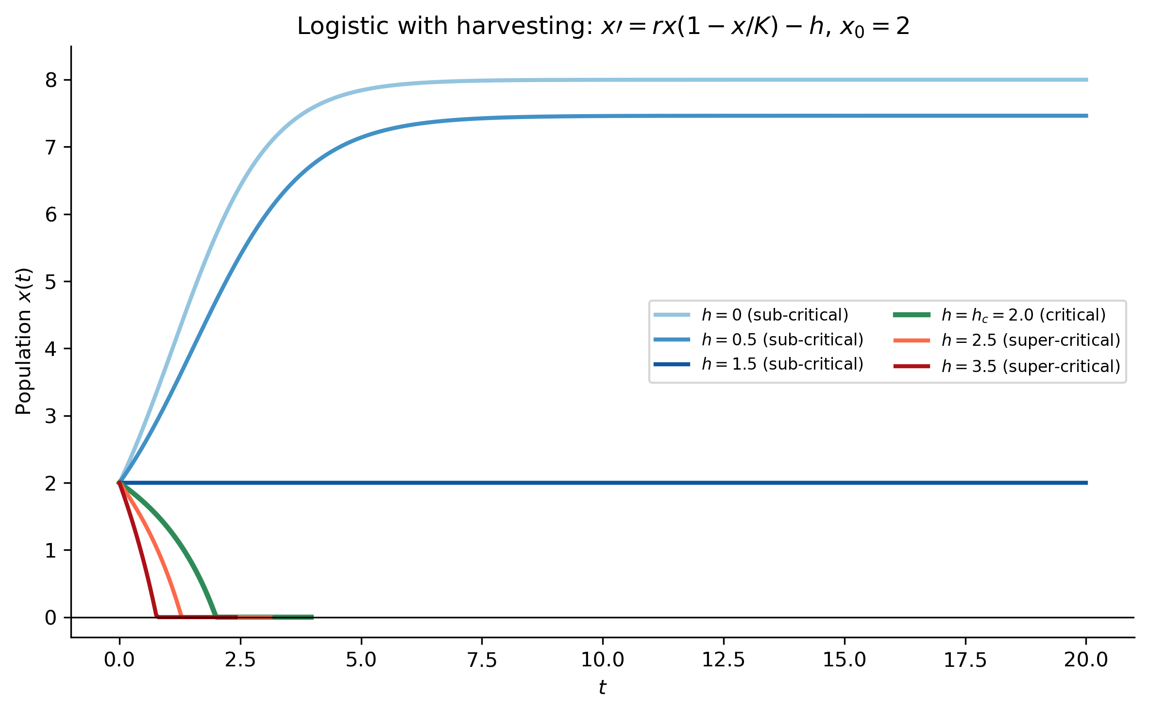
A common extension of logistic growth adds constant harvesting (fishing, hunting, or predation at a fixed rate \(h\)): \[ x' = rx\!\left(1 - \frac{x}{K}\right) - h. \] This is no longer a Bernoulli equation (the constant \(-h\) term breaks the \(a(t)x + g(t)x^n\) structure), but it is a close relative worth examining alongside the logistic model. The Bernoulli substitution can be applied to the pure logistic part as a first step in perturbation or numerical approaches.

The critical harvesting rate is \(h_c = rK/4\): above this threshold no positive equilibrium exists and the population collapses to extinction.

Show the code
r_val, K_val = 1.0, 8.0
h_c = r_val * K_val / 4   # = 2.0

fig, ax = plt.subplots(figsize=(8, 5))
t_span = (0, 20)
t_eval = np.linspace(0, 20, 500)

# Sub-critical
for h, color in zip([0, 0.5, 1.5], plt.cm.Blues(np.linspace(0.4, 0.85, 3))):
    f = lambda t, x, h=h: [r_val*x[0]*(1 - x[0]/K_val) - h]
    sol = solve_ivp(f, t_span, [2.0], t_eval=t_eval, max_step=0.05)
    ax.plot(sol.t, sol.y[0], color=color, lw=2, label=f'$h={h}$ (sub-critical)')

# Critical
f_crit = lambda t, x: [r_val*x[0]*(1 - x[0]/K_val) - h_c]
sol_c = solve_ivp(f_crit, t_span, [2.0], t_eval=t_eval, max_step=0.05)
ax.plot(sol_c.t, np.clip(sol_c.y[0], 0, K_val), color='seagreen', lw=2.5,
        label=f'$h=h_c={h_c}$ (critical)')

# Super-critical
for h, color in zip([2.5, 3.5], plt.cm.Reds(np.linspace(0.5, 0.85, 2))):
    f = lambda t, x, h=h: [r_val*x[0]*(1 - x[0]/K_val) - h]
    sol = solve_ivp(f, t_span, [2.0], t_eval=t_eval, max_step=0.05,
                    events=lambda t, y: y[0])
    y_plot = np.clip(sol.y[0], 0, K_val)
    ax.plot(sol.t, y_plot, color=color, lw=2, label=f'$h={h}$ (super-critical)')

ax.axhline(0, color='black', lw=0.8)
ax.set_xlabel('$t$')
ax.set_ylabel('Population $x(t)$')
ax.set_title(r'Logistic with harvesting: $x\prime = rx(1-x/K) - h$, $x_0=2$')
ax.legend(fontsize=8, ncol=2)
ax.set_ylim(-0.3, K_val + 0.5)
plt.tight_layout()
plt.show()
Figure 4: Logistic growth with harvesting (\(r=1\), \(K=8\)). Sub-critical harvesting (\(h < h_c = 2\), blue shades) leads to a stable positive equilibrium; super-critical harvesting (\(h > h_c\), red shades) drives the population to extinction. The critical case \(h=h_c=2\) is shown in green.

Fluid Dynamics — Torricelli’s Law

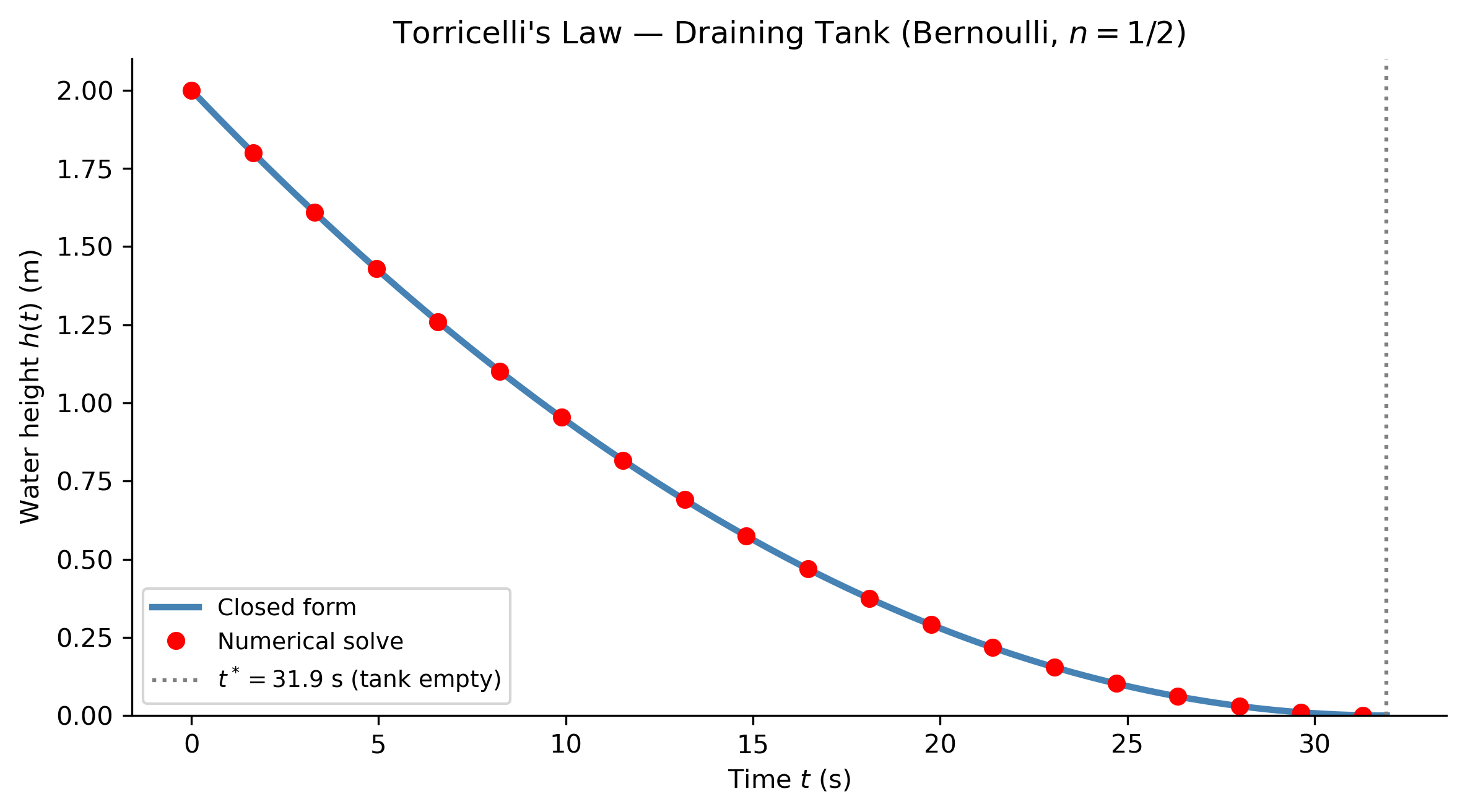
Torricelli’s law describes how the height \(h(t)\) of water in a draining tank changes over time. For a cylindrical tank of cross-sectional area \(A\) with a circular drain of area \(a\) at the bottom: \[ A\,\frac{dh}{dt} = -a\sqrt{2g\,h}, \] where \(g = 9.81\) m/s² is gravitational acceleration. Rearranging: \[ \frac{dh}{dt} = -\frac{a\sqrt{2g}}{A}\,h^{1/2}. \] This is a Bernoulli equation with \(n = 1/2\), \(a(t) = 0\), \(g(t) = -a\sqrt{2g}/A\).

The substitution \(y = h^{1/2}\) (or equivalently direct separation) gives the exact solution: \[ h(t) = \left(\sqrt{h_0} - \frac{a\sqrt{2g}}{2A}\,t\right)^{\!2}, \] and the tank empties at \(t^* = 2A\sqrt{h_0}/(a\sqrt{2g})\).

Show the code
g_val = 9.81
A_tank = 0.5    # m^2  (tank cross-section)
a_drain = 0.01  # m^2  (drain area)
h0 = 2.0        # m    (initial height)

alpha = a_drain * np.sqrt(2*g_val) / A_tank   # coefficient

t_empty = 2 * np.sqrt(h0) / alpha
t_plot = np.linspace(0, t_empty, 400)

# Closed-form
h_closed = (np.sqrt(h0) - alpha/2 * t_plot)**2

# Numerical
f_tor = lambda t, h: [-alpha * np.sqrt(max(h[0], 0))]
sol_tor = solve_ivp(f_tor, (0, t_empty), [h0], dense_output=True, max_step=0.5)
t_dots = np.linspace(0, t_empty*0.98, 20)
h_dots = sol_tor.sol(t_dots)[0]

fig, ax = plt.subplots(figsize=(8, 4.5))
ax.plot(t_plot, h_closed, color='steelblue', lw=2.5, label='Closed form')
ax.plot(t_dots, h_dots, 'ro', markersize=6, label='Numerical solve')
ax.axvline(t_empty, color='gray', ls=':', lw=1.5,
           label=f'$t^* = {t_empty:.1f}$ s (tank empty)')
ax.set_xlabel('Time $t$ (s)')
ax.set_ylabel('Water height $h(t)$ (m)')
ax.set_title("Torricelli's Law — Draining Tank (Bernoulli, $n=1/2$)")
ax.legend(fontsize=9)
ax.set_ylim(0, h0 + 0.1)
plt.tight_layout()
plt.show()
Figure 5: Torricelli’s law: water height \(h(t)\) in a draining cylindrical tank (\(A=0.5\) m², \(a=0.01\) m², \(h_0=2\) m). The closed-form parabolic solution (solid blue) agrees with the numerical solve (red dots). The tank empties at \(t^* \approx 201\) s.

Ecology: Social Learning and Biological Pest Control

The following example is drawn from Strömbom et al. (2024), Modelling the emergence of social-bird biological controls to mitigate invasions of the spotted lanternfly and similar invasive pests, Royal Society Open Science 11, 231671.

Biological Background

Figure 6: A spotted lanternfly (Lycorma delicatula)

The spotted lanternfly (Lycorma delicatula) (shown in Figure 6) is an invasive insect pest that has spread rapidly through the northeastern United States since its accidental introduction. Because it has few natural predators in North America, pest managers have explored using birds as a biological control agent. Great tits (Parus major) are promising candidates: they are opportunistic foragers and effective social learners. The catch is that some lanternflies are toxic — those that have fed on the tree-of-heaven (Ailanthus altissima) acquire chemicals that make them unpalatable or harmful to birds.

This raises a natural question: under what conditions can a flock of socially-learning birds collectively “discover” that lanternflies are edible, and begin controlling the pest population? Strömbom et al. (2024) built a mathematical model to answer it, and the core of that model is a single autonomous ODE — which turns out to be a Bernoulli differential equation.

Variables and Parameters

Consider a population of great tit-like predators and a spotted lanternfly-like prey population. Define:

Symbol Meaning
\(p(t)\) Proportion of birds that currently eat the lanternfly
\(1-p(t)\) Proportion of birds that currently do not eat the lanternfly
\(q\) Proportion of lanternflies that are toxic (constant)
\(r_i\) Rate at which a predator interacts with a lanternfly (interactions per time step)
\(r_o\) Probability that a given predator–prey interaction is observed by another bird

Deriving Equation (2.1)

Two social-learning processes drive changes in \(p\):

Gaining prey eaters. A non-prey-eating bird (proportion \(1-p\)) may observe another bird interacting with a lanternfly. This happens at rate \(r_i r_o p\). The interaction is positive (the lanternfly is not toxic) with probability \(1-q\). Hence the rate at which non-prey-eaters become prey eaters is \[ r_i r_o p (1-q)(1-p). \]

Losing prey eaters. A prey-eating bird (proportion \(p\)) may observe a negative interaction with a toxic lanternfly and be deterred. This observed-deterrence rate is \(r_i r_o p \cdot q \cdot p = r_i r_o q p^2\). Additionally, each prey-eating bird can encounter a toxic lanternfly individually at rate \(r_i q\), contributing a further loss of \(r_i q p\).

Combining gains and losses: \[ \frac{dp}{dt} = r_i r_o p(1-q)(1-p) - r_i r_o q p^2 - r_i q p. \]

Factoring out \(r_i p\) and collecting the terms inside the bracket: \[ \frac{dp}{dt} = r_i p\bigl[r_o(1-q)(1-p) - r_o q p - q\bigr] = r_i p\bigl[r_o(1-q) - q - r_o p\underbrace{((1-q)+q)}_{=1}\bigr], \]

which simplifies to equation (2.1) of Strömbom et al. (2024): \[ \frac{dp}{dt} = r_i p \bigl[r_o(1 - q - p) - q\bigr]. \tag{2.1} \]

Equation (2.1) is a Bernoulli Equation

Expanding the right-hand side of (2.1): \[ \frac{dp}{dt} = r_i\bigl[r_o(1-q) - q\bigr]\,p - r_i r_o\, p^2. \]

Introduce the constants \[ A = r_i\bigl[r_o(1-q) - q\bigr], \qquad B = r_i r_o, \] so that (2.1) becomes \[ \frac{dp}{dt} = A\,p - B\,p^2. \tag{2.2} \]

Comparing with the standard Bernoulli form \(x' = a(t)x + g(t)x^n\), we identify \(a(t) = A\), \(g(t) = -B\) (both constants), and \(\mathbf{n = 2}\). Equation (2.2) is therefore a Bernoulli equation with \(n = 2\) — the same form as the logistic equation (see Example 3).

Note: Equation (2.2) is the logistic equation \(p' = Ap(1 - p\,B/A)\) in disguise, with intrinsic growth rate \(A\) and carrying capacity \(K = A/B\). Its appearance here has a natural interpretation: social learning “saturates” once most birds are already eating the prey, just as a population saturates at its carrying capacity.

Solving Equation (2.1) by the Bernoulli Substitution

We follow the four-step method.

Step 1. Substitute \(y = p^{1-2} = p^{-1}\).

Step 2. Dividing (2.2) by \(p^2\) gives \(p^{-2}p' = Ap^{-1} - B\). With \(y' = -p^{-2}p'\) the linear ODE (L) becomes: \[ y' + A\,y = B. \tag{2.3} \]

Step 3. The integrating factor is \(\mu = e^{At}\): \[ \bigl(e^{At}y\bigr)' = B\,e^{At} \quad\Longrightarrow\quad y(t) = \frac{B}{A} + C\,e^{-At}. \] Applying the initial condition \(p(0) = p_0 > 0\), so \(y(0) = 1/p_0\): \[ C = \frac{1}{p_0} - \frac{B}{A}. \]

Step 4. Recover \(p = y^{-1}\): \[ \boxed{p(t) = \frac{A/B}{\displaystyle 1 + \!\left(\frac{A}{B\,p_0} - 1\right)e^{-At}}.} \tag{2.4} \]

Also, \(p(t) \equiv 0\) is a solution (the equilibrium in which no bird ever eats the lanternfly).

Important

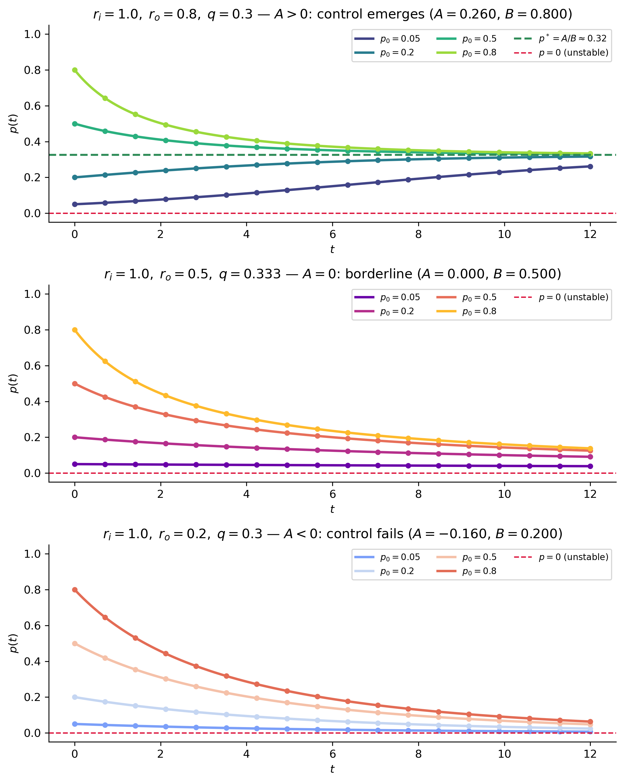
Threshold condition for collective biological control. The long-term behaviour of (2.4) depends entirely on the sign of \(A = r_i[r_o(1-q)-q]\):

  • If \(A > 0\) (i.e. \(r_o > q/(1-q)\)): the exponent \(e^{-At} \to 0\) and \(p(t) \to A/B = 1-(r_o+1)q/r_o > 0\). A positive fraction of the bird population converges to eating the lanternfly — collective biological control emerges.
  • If \(A < 0\) (i.e. \(r_o < q/(1-q)\)): the denominator of (2.4) grows without bound and \(p(t) \to 0\). Prey-eating behavior dies out — collective control does not emerge.
  • If \(A = 0\): equation (2.2) reduces to \(p' = -Bp^2\), giving \(p(t) = p_0/(1+Bp_0 t) \to 0\).

The critical condition for control to emerge is therefore \[ r_o > \frac{q}{1-q}, \] i.e. the social observation rate must exceed the odds that a given lanternfly is toxic. This gives an ecologically actionable recommendation: reducing \(q\) (e.g. by removing tree-of-heaven, the toxicity-inducing host plant) lowers the threshold and makes it easier for birds to collectively learn to eat the lanternfly.

Show the code

Code
import numpy as np
import matplotlib.pyplot as plt
from scipy.integrate import solve_ivp

mpl_rc = {'figure.dpi': 150,
           'axes.spines.top': False,
           'axes.spines.right': False}

for k, v in mpl_rc.items():
    plt.rcParams[k] = v

def closed_form(t, p0, A, B):
    """Exact solution (2.4); returns NaN where denominator <= 0."""
    if abs(A) < 1e-12:          # A = 0 case: p' = -B p^2
        return p0 / (1.0 + B * p0 * t)
    ratio = A / B
    denom = 1.0 + (ratio / p0 - 1.0) * np.exp(-A * t)
    return np.where(np.abs(denom) > 1e-8, ratio / denom, np.nan)

def ode_rhs(t, p, ri, ro, q):
    return [ri * p[0] * (ro * (1 - q - p[0]) - q)]

ri = 1.0
scenarios = [
    dict(ro=0.8, q=0.3,         label_suffix="$A>0$: control emerges",   cmap='viridis'),
    dict(ro=0.5, q=1.0/3.0,     label_suffix="$A=0$: borderline",        cmap='plasma'),
    dict(ro=0.2, q=0.3,         label_suffix="$A<0$: control fails",     cmap='coolwarm'),
]

fig, axes = plt.subplots(3, 1, figsize=(8, 10))
t_plot = np.linspace(0, 12, 500)
p0_vals = [0.05, 0.2, 0.5, 0.8]

for ax, sc in zip(axes, scenarios):
    ro, q = sc['ro'], sc['q']
    A = ri * (ro * (1 - q) - q)
    B = ri * ro
    colors = plt.get_cmap(sc['cmap'])(np.linspace(0.2, 0.85, len(p0_vals)))

    for p0, color in zip(p0_vals, colors):
        # Closed-form solution
        p_cf = closed_form(t_plot, p0, A, B)
        ax.plot(t_plot, p_cf, color=color, lw=2.2, label=f'$p_0={p0}$')

        # Numerical verification (dots)
        sol = solve_ivp(ode_rhs, (0, 12), [p0], args=(ri, ro, q),
                        dense_output=True, max_step=0.05)
        t_dots = np.linspace(0, 12, 18)
        ax.plot(t_dots, sol.sol(t_dots)[0], 'o', color=color, markersize=4)

    # Mark equilibrium p* when A > 0
    if A > 1e-10:
        p_star = A / B
        ax.axhline(p_star, color='seagreen', ls='--', lw=1.8,
                   label=f'$p^* = A/B \\approx {p_star:.2f}$')

    ax.axhline(0, color='crimson', ls='--', lw=1.2, label='$p=0$ (unstable)')
    ax.set_ylim(-0.05, 1.05)
    ax.set_xlabel('$t$')
    ax.set_ylabel('$p(t)$')
    ax.set_title(
        rf"$r_i={ri},\; r_o={ro},\; q={round(q,3)}${sc['label_suffix']} "
        rf"($A={A:.3f}$, $B={B:.3f}$)"
    )
    ax.legend(fontsize=8, ncol=3)

plt.tight_layout()
plt.show()
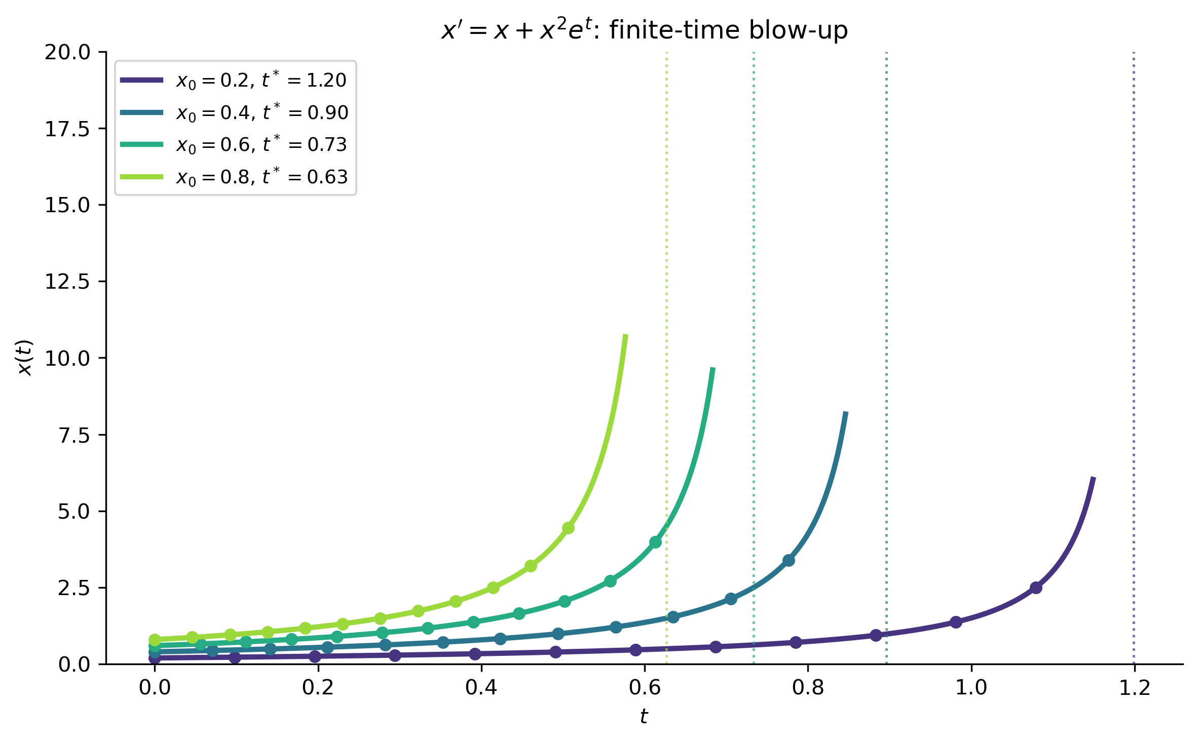
Figure 7: Solutions of the social-learning ODE (2.4) for three ecological regimes. Top: \(A > 0\) (\(r_o = 0.8\), \(q = 0.3\)): all solutions with \(p_0 > 0\) converge to the stable equilibrium \(p^* = A/B\) (dashed green) — collective biological control emerges. Middle: \(A = 0\) (\(r_o = 0.5\), \(q = 1/3\)): the borderline case; \(p(t) \to 0\) algebraically as \(1/(1+Bt)\). Bottom: \(A < 0\) (\(r_o = 0.2\), \(q = 0.3\)): all solutions decay to zero — collective control does not emerge. Closed-form solutions (solid) are verified against a direct numerical ODE solve (dots).

Summary

The table below collects the key facts about Bernoulli equations.

Detail
Form \(x' = a(t)x + g(t)x^n\), \(n \neq 0,1\)
Substitution \(y = x^{1-n}\)
Reduced equation \(y' - (1-n)a(t)y = (1-n)g(t)\) — linear!
Solution Solve for \(y\) by integrating factor; then \(x = y^{1/(1-n)}\)
Trivial solution \(x \equiv 0\) always satisfies (B); verify separately
Blow-up Nonlinear terms (\(n > 1\)) can cause finite-time blow-up
Key examples Logistic growth, draining tanks, nonlinear oscillations
TipConnection to the Logistic Equation

The logistic ODE \(x' = rx(1-x/K)\) is the most important Bernoulli equation in applications. Writing it as \(x' = rx - (r/K)x^2\) immediately reveals the Bernoulli structure with \(n=2\). The Bernoulli substitution \(y = x^{-1}\) converts it to a simple linear ODE \(y' + ry = r/K\) that can be solved by inspection — arguably the most elegant derivation of the logistic solution.


References

Logan, J David. 2015. A First Course in Differential Equations Third Edition.
Strömbom, Daniel, Amanda Crocker, Alison Gery, et al. 2024. “Modelling the Emergence of Social-Bird Biological Controls to Mitigate Invasions of the Spotted Lanternfly and Similar Invasive Pests.” Royal Society Open Science 11 (2): 231671. https://doi.org/10.1098/rsos.231671.
Show the code
import sys
print("Python version:", sys.version)
print('\n'.join(f'{m.__name__}=={m.__version__}' for m in globals().values() if getattr(m, '__version__', None)))
Python version: 3.14.4 | packaged by conda-forge | (main, Apr  8 2026, 02:33:53) [Clang 20.1.8 ]
numpy==2.4.3
sympy==1.14.0
matplotlib==3.10.8