import numpy as npimport sympy as symimport matplotlib as mplimport matplotlib.pyplot as pltfrom scipy.integrate import solve_ivpfrom IPython.display import Math, displaympl.rcParams['figure.dpi'] =150mpl.rcParams['axes.spines.top'] =Falsempl.rcParams['axes.spines.right'] =False
This section provides a deeper look at the classical mechanics background for the second-order linear ODEs studied in Chapter 2 of (Logan 2015), corresponding to Section 2.1. We develop the spring–mass system from first principles — deriving the governing ODE from Newton’s second law and Hooke’s law — analyze the three damping regimes in detail, investigate energy conservation and dissipation, and conclude with a discussion of forced oscillations and resonance from a physical perspective. The mechanical– electrical analogy, which shows that RLC circuits obey the same mathematics, is highlighted throughout.
The material here supplements and expands upon (Logan 2015) §2.1 and connects directly to the solution methods of §2.2–2.3 covered in Notes 4.
Newton’s Second Law and the Program of Classical Mechanics
\[
F = ma \quad\Longleftrightarrow\quad m\,x'' = F(t, x, x'),
\]
where \(x(t)\) is the position of a particle of mass \(m\), \(x'\) is its velocity, \(x''\) its acceleration, and \(F\) is the total external force (which may depend on time, position, and velocity).
For a mechanical system we always impose two initial conditions, \[
x(0) = x_0 \quad\text{(initial position)}, \qquad x'(0) = v_0 \quad\text{(initial velocity)},
\] making this an initial value problem (IVP) for a second-order ODE.
ImportantDeterminism in Classical Mechanics
The Picard–Lindelöf theorem guarantees that — under mild smoothness conditions on \(F\) — the IVP has a unique solution. This is the mathematical expression of Laplacian determinism: knowing the complete state \((x_0, v_0)\) of a particle at one instant, together with all the forces acting on it, uniquely determines its entire future (and past) motion. This was the philosophical bedrock of 18th- and 19th-century physics.
The Spring–Mass System
Setup and Free-Body Diagram
Consider a mass \(m\) on a frictionless horizontal surface, attached to a spring of natural length \(\ell_0\) with spring constant \(k > 0\), the other end fixed to a wall. We measure the displacement \(x(t)\) from the equilibrium position (where the spring is neither stretched nor compressed), with \(x > 0\) to the right.
Hooke’s law states that for small displacements the spring exerts a restoring force proportional to the displacement: \[
F_s = -kx.
\] The minus sign is essential: the spring always pulls the mass back toward equilibrium.
NoteJustification of Hooke’s Law via Taylor Expansion
If we allow the spring force \(F_s = F_s(x)\) to be any smooth function of displacement with \(F_s(0) = 0\), then by Taylor’s theorem: \[
F_s(x) = F_s(0) + F_s'(0)\,x + \tfrac{1}{2}F_s''(0)\,x^2 + \cdots = -kx + O(x^2),
\] where \(k = -F_s'(0) > 0\). Hooke’s law is the linear approximation valid for small displacements. It is an empirical constitutive relation — a model for springs, not a law of nature — and breaks down for large displacements or non-linear springs.
Applying Newton’s second law: \[
m\,x'' = F_s = -kx \quad\Longrightarrow\quad \boxed{m\,x'' + kx = 0.}
\] Dividing by \(m\) and setting \(\omega_0 = \sqrt{k/m}\) (the natural angular frequency): \[
x'' + \omega_0^2\,x = 0. \tag{SHO}
\] This is the simple harmonic oscillator (SHO) equation.
Measuring the Spring Constant
A practical way to determine \(k\): hang the spring vertically, attach mass \(m\), and measure the static elongation \(\Delta L\). At equilibrium, gravity \(mg\) (downward) balances the spring restoring force \(k\Delta L\) (upward): \[
mg = k\Delta L \quad\Longrightarrow\quad k = \frac{mg}{\Delta L}.
\]
Show the code
g =9.81# m/s^2for m_kg, DL_m in [(0.3, 0.05), (0.5, 0.08), (1.0, 0.12)]: k = m_kg * g / DL_m omega0 = np.sqrt(k / m_kg) period =2* np.pi / omega0print(f"m={m_kg} kg, ΔL={DL_m} m: k={k:.2f} N/m, ω₀={omega0:.3f} rad/s, T={period:.3f} s")
m=0.3 kg, ΔL=0.05 m: k=58.86 N/m, ω₀=14.007 rad/s, T=0.449 s
m=0.5 kg, ΔL=0.08 m: k=61.31 N/m, ω₀=11.074 rad/s, T=0.567 s
m=1.0 kg, ΔL=0.12 m: k=81.75 N/m, ω₀=9.042 rad/s, T=0.695 s
The General Solution of the SHO
The characteristic equation of (SHO) is \(\lambda^2 + \omega_0^2 = 0\), giving pure imaginary eigenvalues \(\lambda = \pm i\omega_0\). The general solution is: \[
x(t) = C_1\cos(\omega_0 t) + C_2\sin(\omega_0 t).
\] This can equivalently be written in amplitude-phase form: \[
\boxed{x(t) = A\cos(\omega_0 t - \phi),}
\] where the amplitude\(A = \sqrt{C_1^2 + C_2^2}\) and the phase\(\phi = \arctan(C_2/C_1)\) are determined by the initial conditions: \[
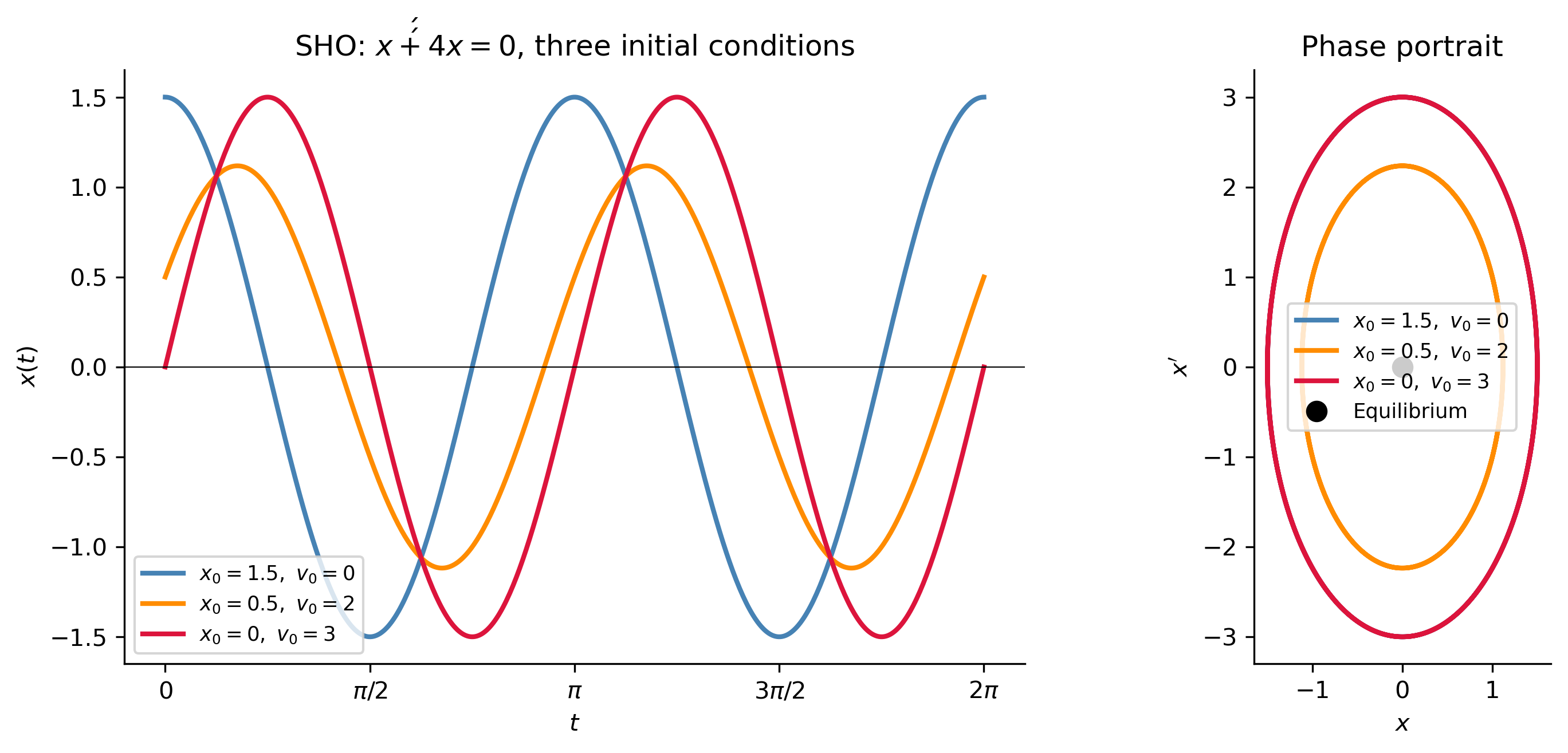
C_1 = x_0, \qquad C_2 = \frac{v_0}{\omega_0},
\qquad A = \sqrt{x_0^2 + \frac{v_0^2}{\omega_0^2}}.
\]
Key properties of the SHO:
Quantity
Formula
Physical meaning
Natural frequency
\(\omega_0 = \sqrt{k/m}\)
Radians per second
Period
\(T = 2\pi/\omega_0 = 2\pi\sqrt{m/k}\)
Time for one full oscillation
Frequency
\(f = 1/T = \omega_0/(2\pi)\)
Oscillations per second (Hz)
Amplitude
\(A = \sqrt{x_0^2 + v_0^2/\omega_0^2}\)
Maximum displacement
Tip
The period \(T = 2\pi\sqrt{m/k}\) is independent of amplitude — a heavier mass oscillates more slowly, a stiffer spring oscillates faster. This isochronism (equal-time property) was first noted by Galileo for the pendulum (which obeys the same equation for small angles) and is the operating principle behind pendulum clocks.
Figure 1: Simple harmonic oscillator \(x''+4x=0\) (\(\omega_0=2\)). Left: solution curves for three different initial conditions, all with period \(T=\pi\). Right: phase portrait — each closed ellipse is a trajectory; the amplitude \(A=\sqrt{x_0^2+v_0^2/\omega_0^2}\) is conserved. The energy level \(E=\frac{1}{2}kA^2=2A^2\) labels each ellipse.
The Damped Oscillator
In reality, friction, air resistance, and internal material damping dissipate energy from the system. The simplest model takes the damping force proportional to velocity: \[
F_d = -\gamma\,x', \qquad \gamma > 0 \;\text{(damping coefficient, units: kg/s)}.
\] This is a viscous damping model. The minus sign ensures that the damping force always opposes motion.
Applying Newton’s second law with both spring and damping forces: \[
m\,x'' = F_s + F_d = -kx - \gamma x'.
\] Rearranging: \[
\boxed{m\,x'' + \gamma\,x' + kx = 0.} \tag{DO}
\] This is the damped oscillator equation.
Dividing by \(m\) and writing \(2\gamma_m = \gamma/m\) (the damping ratio per unit mass) and \(\omega_0^2 = k/m\): \[
x'' + 2\gamma_m\,x' + \omega_0^2\,x = 0.
\] The characteristic equation is \(\lambda^2 + 2\gamma_m\lambda + \omega_0^2 = 0\), with discriminant \(\Delta = 4(\gamma_m^2 - \omega_0^2)\), yielding the three damping regimes of Notes 4.
The Three Regimes: Physical Interpretation
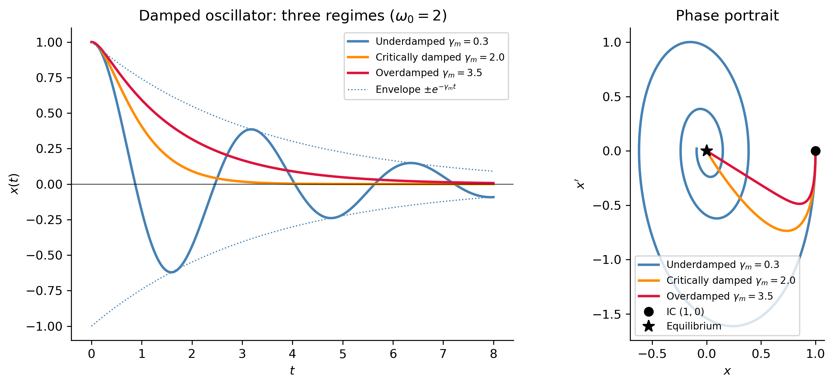
Underdamped (\(\gamma_m < \omega_0\), i.e., \(\gamma < 2\sqrt{mk}\)): \[
x(t) = e^{-\gamma_m t}(C_1\cos\omega_d t + C_2\sin\omega_d t)
= A\,e^{-\gamma_m t}\cos(\omega_d t - \phi),
\] where \(\omega_d = \sqrt{\omega_0^2 - \gamma_m^2}\) is the damped natural frequency. The system oscillates at a slightly lower frequency than the undamped case, with amplitude decaying like \(e^{-\gamma_m t}\).
Critically damped (\(\gamma_m = \omega_0\), i.e., \(\gamma = 2\sqrt{mk}\)): \[
x(t) = (C_1 + C_2 t)\,e^{-\gamma_m t}.
\] No oscillation. The system returns to equilibrium as fast as possible without overshooting. Critical damping is optimal for many engineering applications — door closers, shock absorbers, galvanometers.
Overdamped (\(\gamma_m > \omega_0\), i.e., \(\gamma > 2\sqrt{mk}\)): \[
x(t) = C_1\,e^{\lambda_1 t} + C_2\,e^{\lambda_2 t},
\quad \lambda_{1,2} = -\gamma_m \pm \sqrt{\gamma_m^2 - \omega_0^2} < 0.
\] Both eigenvalues are negative, so the solution decays without oscillation — but more slowly than critically damped because the strong damping impedes motion back to equilibrium.
Figure 2: Damped oscillator \(x''+2\gamma_m x'+4x=0\) (\(\omega_0=2\), \(x(0)=1\), \(x'(0)=0\)). Left: position vs. time for all three regimes. The underdamped case shows decaying oscillations; the dotted envelope \(\pm e^{-\gamma_m t}\) bounds the oscillation amplitude. Right: phase portrait. The underdamped spiral converges to the origin; the overdamped and critically damped cases arrive along the positive-\(x\) axis without orbiting.
Energy: Conservation and Dissipation
Conservation of Energy (Undamped)
For the undamped SHO, multiply the equation \(mx'' + kx = 0\) by \(x'\): \[
m\,x'\,x'' + k\,x\,x' = 0.
\] Using the chain rule \(\frac{d}{dt}(x')^2 = 2x'x''\) and \(\frac{d}{dt}x^2 = 2xx'\): \[
\frac{d}{dt}\!\left[\frac{1}{2}m(x')^2 + \frac{1}{2}kx^2\right] = 0.
\]
ImportantConservation of Energy
For the undamped spring–mass system, \[
E = T + V = \frac{1}{2}m(x')^2 + \frac{1}{2}kx^2 = \text{const},
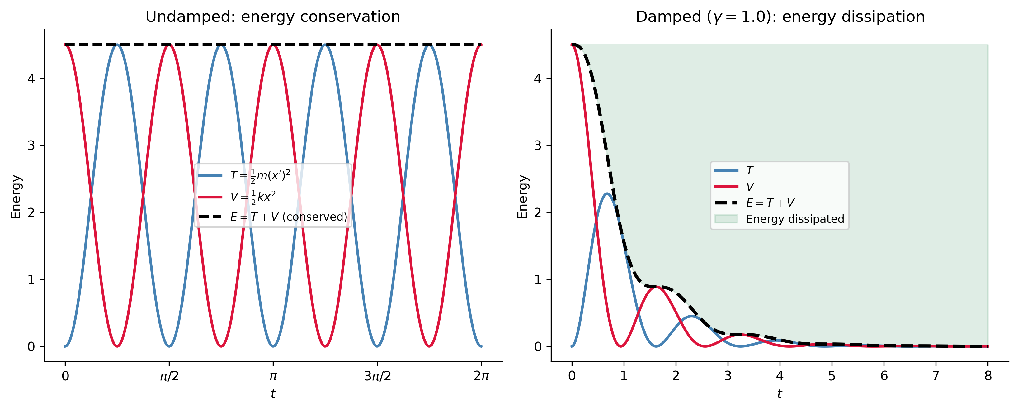
\] where \(T = \frac{1}{2}m(x')^2\) is the kinetic energy and \(V = \frac{1}{2}kx^2\) is the potential energy (elastic energy stored in the spring). Energy oscillates between kinetic and potential but the total is conserved.
The constant \(E\) is determined by the initial conditions: \(E = \frac{1}{2}mv_0^2 + \frac{1}{2}kx_0^2\). The amplitude of oscillation satisfies \(E = \frac{1}{2}kA^2\), giving \(A = \sqrt{2E/k}\).
In the phase plane, the energy conservation law \(E = \frac{1}{2}m(x')^2 + \frac{1}{2}kx^2\) defines an ellipse for each value of \(E\) — these are precisely the closed orbits in the phase portrait.
Energy Dissipation (Damped)
For the damped oscillator, the same multiplication by \(x'\) gives: \[
\frac{d}{dt}\!\left[\frac{1}{2}m(x')^2 + \frac{1}{2}kx^2\right] = -\gamma(x')^2.
\]
ImportantEnergy Dissipation Law
\[
\frac{dE}{dt} = -\gamma(x')^2 \leq 0.
\] The total mechanical energy \(E = T + V\) decreases at a rate equal to the power dissipated by damping. Since \((x')^2 \geq 0\), energy is monotonically non-increasing. The damping force converts mechanical energy to heat.
For the RLC circuit, the analogous equation is \[\frac{d}{dt}\!\left[\frac{1}{2}LI^2 + \frac{Q^2}{2C}\right] = -RI^2,\] where \(\frac{1}{2}LI^2\) is the magnetic energy stored in the inductor, \(Q^2/(2C)\) is the electric energy stored in the capacitor, and \(RI^2\) is the Joule heating power dissipated by the resistor.
Figure 3: Energy in the spring–mass system (\(m=1\), \(k=4\), \(x(0)=1.5\), \(x'(0)=0\)). Left: undamped (\(\gamma=0\)) — total energy \(E\) (black dashed) is constant; kinetic \(T\) and potential \(V\) oscillate out of phase, trading energy back and forth. Right: damped (\(\gamma=1\)) — total energy decays exponentially; the shaded area represents energy dissipated.
The Mechanical–Electrical Analogy
One of the most elegant facts in applied mathematics is that the damped spring–mass equation and the RLC circuit equation are mathematically identical:
The correspondence between mechanical and electrical quantities:
Mechanical
Symbol
Electrical
Symbol
Mass (inertia)
\(m\)
Inductance
\(L\)
Damping coefficient
\(\gamma\)
Resistance
\(R\)
Spring stiffness
\(k\)
Inverse capacitance
\(1/C\)
Position
\(x\)
Charge
\(Q\)
Velocity
\(x'\)
Current
\(I = Q'\)
Applied force
\(F(t)\)
Electromotive force (emf)
\(E(t)\)
Kinetic energy \(\frac{1}{2}mv^2\)
\(T\)
Magnetic energy \(\frac{1}{2}LI^2\)
—
Potential energy \(\frac{1}{2}kx^2\)
\(V\)
Electric energy \(Q^2/2C\)
—
Power dissipated \(\gamma v^2\)
—
Joule heating \(RI^2\)
—
TipWhy the Analogy Matters
This analogy is not merely a curiosity. It means that every mathematical result derived for one system applies immediately to the other. Engineers routinely build analog electrical circuits to simulate mechanical systems — before digital computers, this was the standard way to study the dynamics of aircraft, ships, and engines. The analogy also shows that mathematics unifies apparently different physical domains under the same abstract structure.
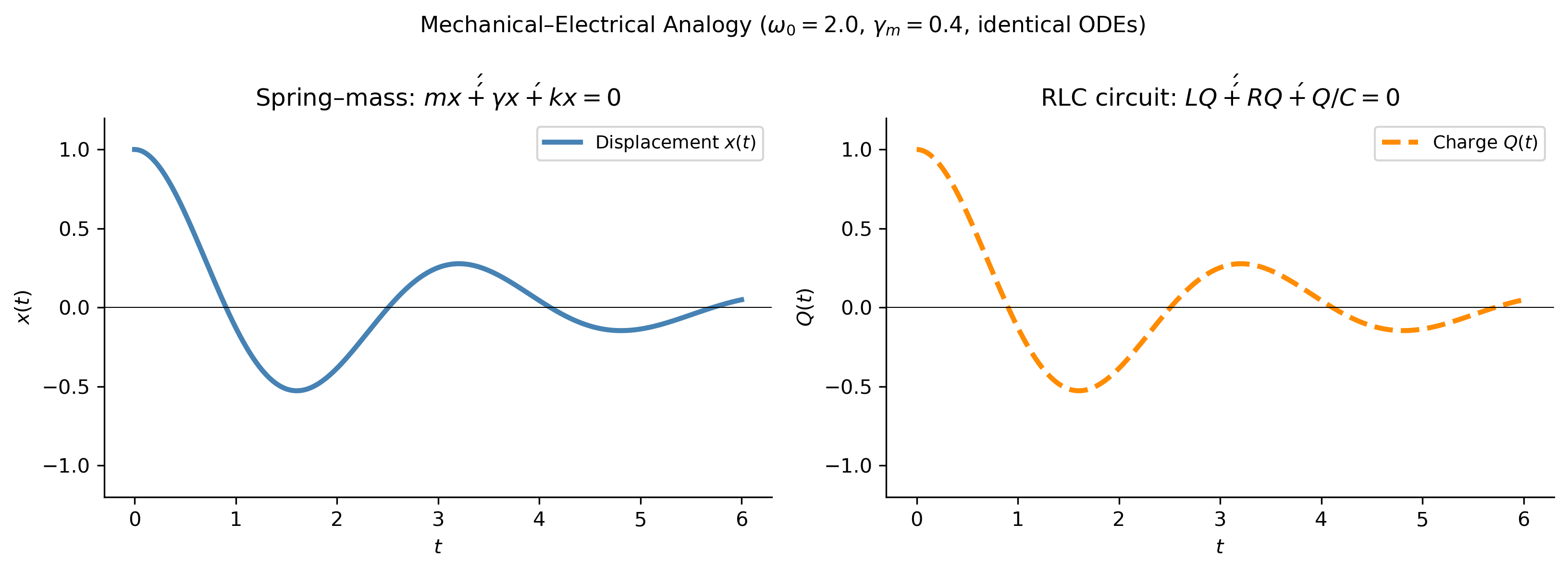
Figure 4: The mechanical–electrical analogy. Spring–mass (left) and RLC circuit (right) obey identical ODEs. The simulation shows \(x(t)\) for the mechanical system (blue) and \(Q(t)\) for the circuit (orange dashed) with matching dimensionless parameters \(\omega_0=2\), \(\gamma_m=0.4\), both starting from the same initial conditions. The curves are identical — up to the choice of units.
Forced Oscillations and Resonance
Adding an External Force
In many applications the spring–mass system is subjected to an external periodic force\(F(t) = F_0\cos(\Omega t)\) (from an engine, an earthquake, a loudspeaker, etc.). The equation of motion becomes:
Here \(\Omega\) is the driving frequency (set externally) and \(\omega_0 = \sqrt{k/m}\) is the natural frequency (set by the system). The long-time behavior is governed by the particular solution — the steady-state response — which oscillates at the driving frequency \(\Omega\).
The Steady-State Amplitude
By the method of undetermined coefficients (Notes 4), the steady-state solution of (FO) is: \[
x_p(t) = G(\Omega)\cos(\Omega t - \phi),
\] where the amplitude response function is: \[
G(\Omega) = \frac{F_0/m}{\sqrt{(\omega_0^2 - \Omega^2)^2 + (2\gamma_m\Omega)^2}}.
\]
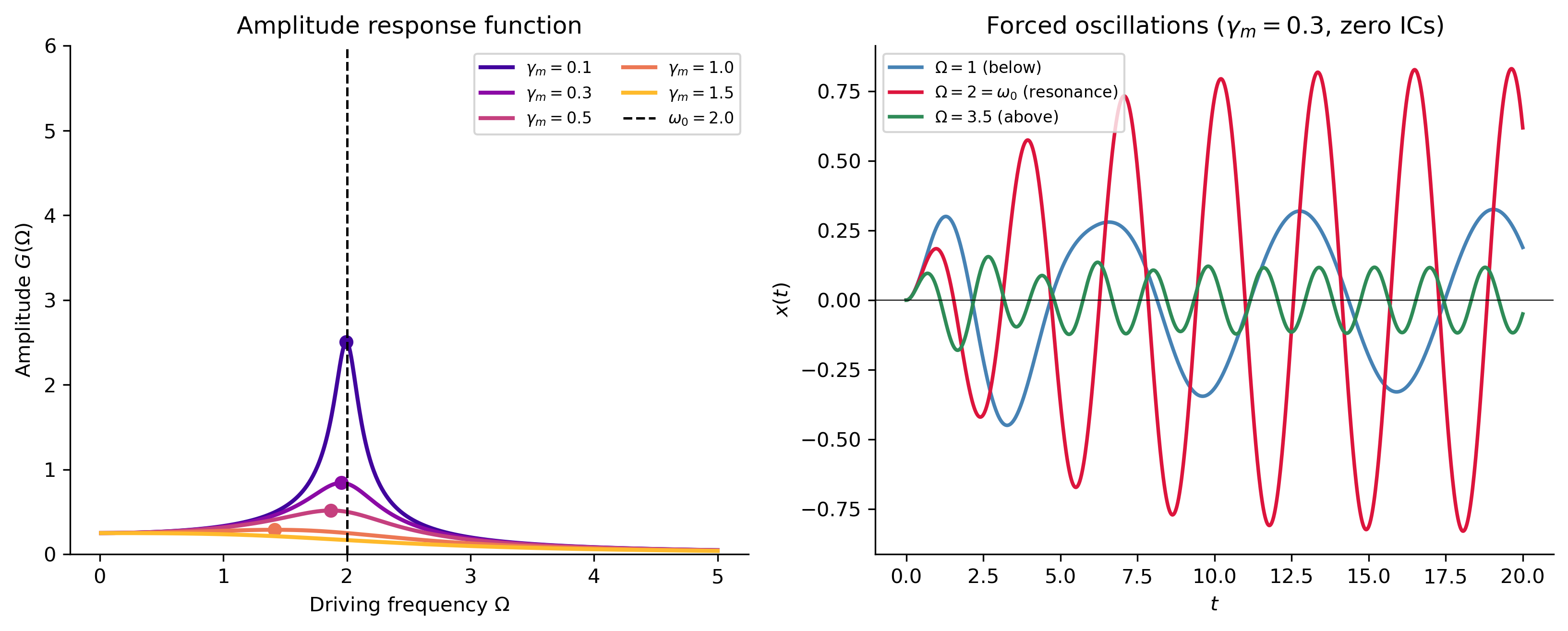
This function is large when \(\Omega \approx \omega_0\) and the damping is small — this is resonance.
ImportantResonance (Undamped Case)
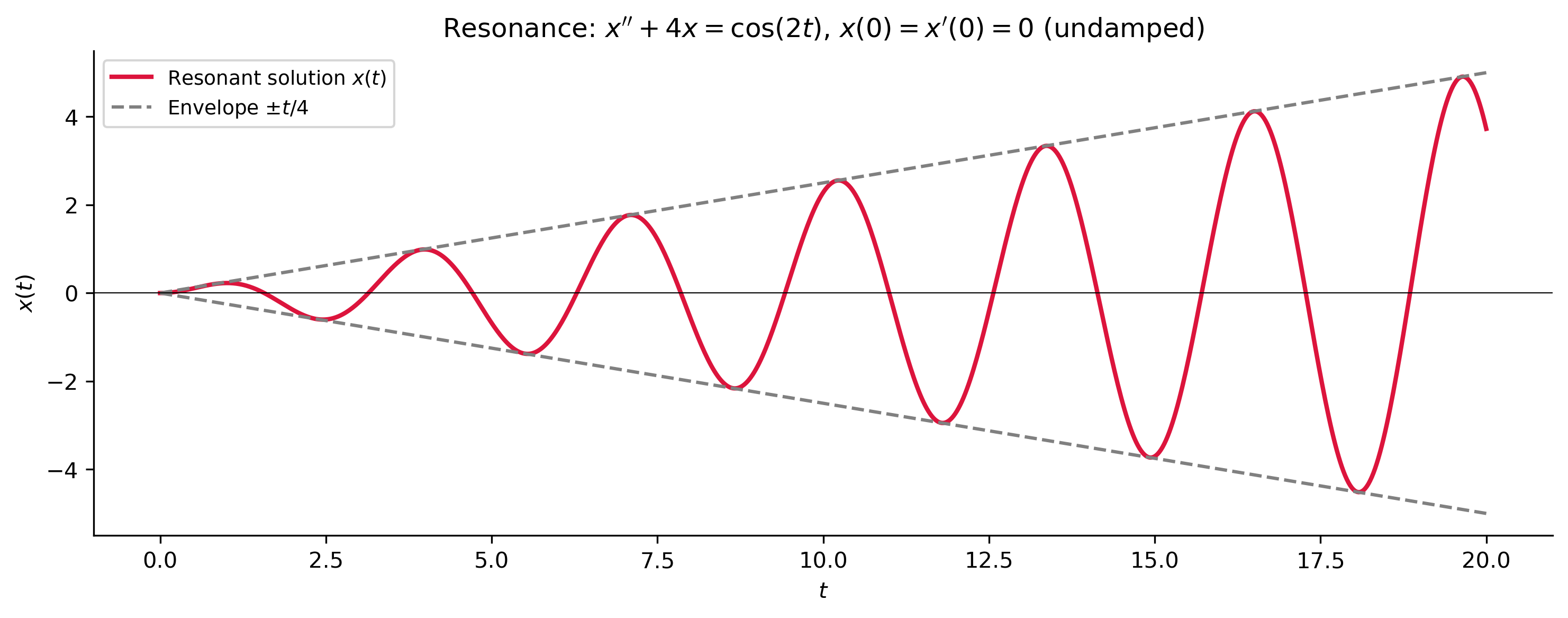
When \(\gamma = 0\) and \(\Omega = \omega_0\), the particular solution is: \[x_p(t) = \frac{F_0}{2m\omega_0}\,t\sin(\omega_0 t).\] The amplitude grows linearly without bound — physical resonance.
The resonant frequency (peak of \(G\)) for the damped system is: \[
\Omega_{\rm res} = \sqrt{\omega_0^2 - 2\gamma_m^2} < \omega_0,
\] which is slightly below the natural frequency.
Figure 5: Frequency response of the forced damped oscillator (\(\omega_0=2\), \(F_0/m=1\)). Left: amplitude \(G(\Omega)\) vs. driving frequency for several damping ratios. The peak shifts below \(\omega_0=2\) (vertical dashed line) and broadens as damping increases. Right: time-domain steady-state solutions for three driving frequencies with \(\gamma_m=0.3\), illustrating below-resonance, at-resonance, and above-resonance behavior.
Resonance in Engineering and Nature
Resonance is one of the most important phenomena arising from second-order linear ODEs, with consequences ranging from catastrophic to beneficial.
Mechanical fatigue: repeated forcing near resonance builds up stress amplitude, eventually causing fracture even when each individual loading is far below the static failure load.
MRI scanners: radio-frequency pulses are tuned to the resonant frequency of nuclear spins (\(\omega_0 = \gamma B_0\), where \(B_0\) is the magnetic field strength and \(\gamma\) is the gyromagnetic ratio).
Musical instruments: the resonant frequencies of strings, air columns, and membranes determine the pitches of notes.
Radio tuning: a variable capacitor adjusts \(\omega_0 = 1/\sqrt{LC}\) to match the carrier frequency of the desired station.
Quartz oscillators: the precise resonant frequency of a quartz crystal (in the MHz range) drives digital clocks and computers.
Figure 6: Resonance amplitude buildup (\(\omega_0=2\), \(\gamma=0\), zero ICs). Without damping, the resonant particular solution \(x_p = (t/4)\sin(2t)\) grows linearly without bound (dashed line shows the envelope \(\pm t/4\)). In practice, material nonlinearities or structural failure occur before infinite amplitude is reached.
The Vertical Spring–Mass System
It is natural to ask whether the spring–mass equation changes when the spring is oriented vertically (e.g., a mass hanging from a spring attached to the ceiling). The answer is no — the equation of motion is identical.
Derivation. Let \(y\) measure displacement from the ceiling attachment point (downward positive). At the unstretched length \(L\) of the spring the mass is at position \(y=L\). At the static equilibrium position \(y = L + \Delta L\), gravity \(mg\) balances the spring force \(k\Delta L\): \[k\Delta L = mg.\] Let \(x = y - (L + \Delta L)\) measure displacement from equilibrium. Then: \[
m\,x'' = mg - k(x + \Delta L) = mg - kx - k\Delta L = -kx,
\] since \(k\Delta L = mg\). The gravitational term cancels exactly, and we recover \(mx'' + kx = 0\) — gravity does not appear in the equation of motion about the equilibrium position.
TipPhysical Insight
Gravity merely shifts the equilibrium position downward by \(\Delta L = mg/k\). Measuring from this new equilibrium, the oscillation is governed by the same SHO equation. The spring carries gravity “for free.” This is why pendulum clocks tick at the same rate regardless of whether they hang vertically or (approximately) on a tilted wall.
Summary
Concept
Formula
Physical meaning
Newton’s second law
\(mx'' = F(t,x,x')\)
Governs all particle motion
SHO
\(x'' + \omega_0^2 x = 0\), \(\omega_0=\sqrt{k/m}\)