Linear Algebra for Applications

Vectors, Matrices, Eigenvalues, and Applications

Show the code
import numpy as np
import sympy as sym
import matplotlib as mpl
import matplotlib.pyplot as plt
from scipy.linalg import solve, lu, qr, svd, norm, lstsq
from IPython.display import Math, display
mpl.rcParams['figure.dpi'] = 150
mpl.rcParams['axes.spines.top'] = False
mpl.rcParams['axes.spines.right'] = False

Linear algebra is the mathematical language of data, networks, signals, structures, and systems. While this course focuses primarily on differential equations, the two subjects are deeply intertwined: the solution of linear ODEs depends on eigenvalues and eigenvectors, and the numerical solution of any system of equations — differential or otherwise — ultimately reduces to linear algebra.

This section presents the core concepts of real linear algebra from first principles, develops facility with NumPy and SymPy as computational tools, and then explores a range of engineering applications that are entirely independent of differential equations.


Part 1 — Vectors in \(\mathbb{R}^n\)

Basic Operations

A vector in \(\mathbb{R}^n\) is an ordered list of \(n\) real numbers: \[\mathbf{u} = \begin{pmatrix}u_1\\ u_2\\ \vdots\\ u_n\end{pmatrix}.\]

Two fundamental operations:

  • Addition: \(\mathbf{u}+\mathbf{v} = (u_1+v_1,\ldots,u_n+v_n)^T\)
  • Scalar multiplication: \(c\mathbf{u} = (cu_1,\ldots,cu_n)^T\)

These satisfy the eight axioms that define a vector space.

The Dot Product and Geometry

The dot product (inner product) of \(\mathbf{u}, \mathbf{v}\in\mathbb{R}^n\) is: \[\mathbf{u}\cdot\mathbf{v} = \sum_{i=1}^n u_i v_i.\]

From this we derive:

Quantity Formula Meaning
Norm (length) \(\|\mathbf{u}\| = \sqrt{\mathbf{u}\cdot\mathbf{u}}\) Distance from origin
Angle \(\cos\theta = \dfrac{\mathbf{u}\cdot\mathbf{v}}{\|\mathbf{u}\|\|\mathbf{v}\|}\) Angle between vectors
Orthogonality \(\mathbf{u}\cdot\mathbf{v} = 0\) Perpendicular
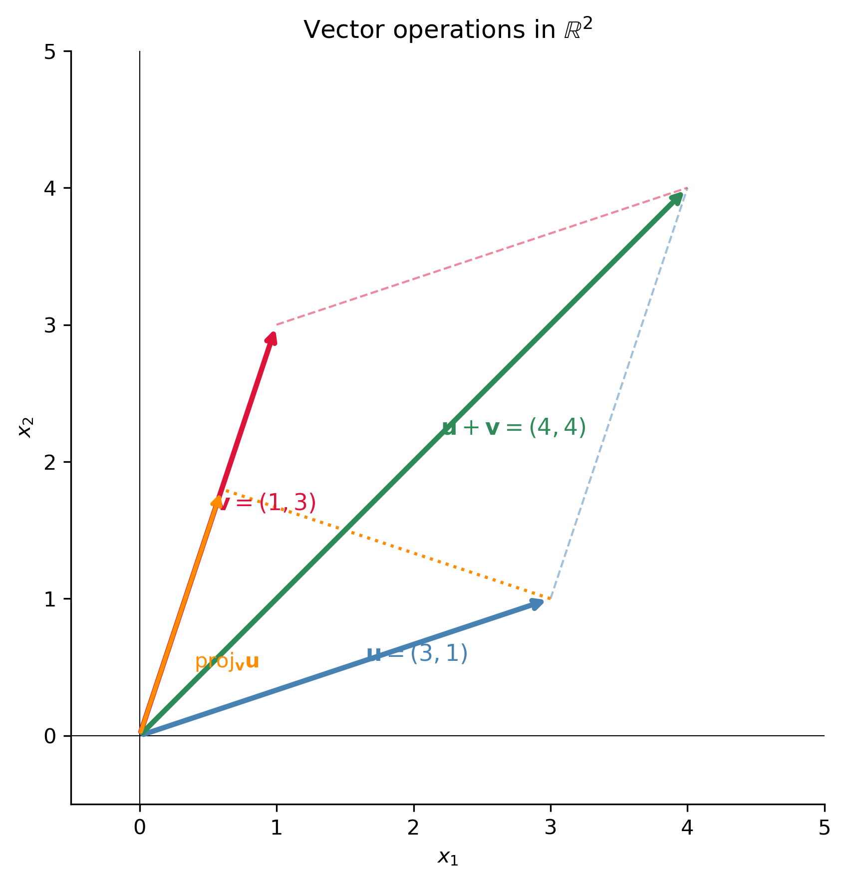
Projection \(\text{proj}_\mathbf{v}\mathbf{u} = \dfrac{\mathbf{u}\cdot\mathbf{v}}{\|\mathbf{v}\|^2}\mathbf{v}\) Shadow of \(\mathbf{u}\) onto \(\mathbf{v}\)

The Cauchy–Schwarz inequality \(|\mathbf{u}\cdot\mathbf{v}| \leq \|\mathbf{u}\|\|\mathbf{v}\|\) guarantees that \(\cos\theta\in[-1,1]\), so the angle is well-defined.

Show the code
u = np.array([3.0, 1.0])
v = np.array([1.0, 3.0])
proj = (np.dot(u,v)/np.dot(v,v)) * v

fig, ax = plt.subplots(figsize=(7, 6))
ax.set_aspect('equal')
ax.axhline(0, color='k', lw=0.5); ax.axvline(0, color='k', lw=0.5)

origin = np.array([0,0])
for vec, color, lbl in [(u,'steelblue','$\\mathbf{u}=(3,1)$'),
                        (v,'crimson','$\\mathbf{v}=(1,3)$'),
                        (u+v,'seagreen','$\\mathbf{u}+\\mathbf{v}=(4,4)$')]:
    ax.annotate('', xy=vec, xytext=origin,
                arrowprops=dict(arrowstyle='->', color=color, lw=2.5))
    ax.text(*(vec*0.55), lbl, color=color, fontsize=11)

# Parallelogram
ax.plot([u[0],u[0]+v[0]], [u[1],u[1]+v[1]], '--', color='steelblue', lw=1, alpha=0.5)
ax.plot([v[0],u[0]+v[0]], [v[1],u[1]+v[1]], '--', color='crimson', lw=1, alpha=0.5)

# Projection
ax.annotate('', xy=proj, xytext=origin,
            arrowprops=dict(arrowstyle='->', color='darkorange', lw=2))
ax.plot([u[0],proj[0]], [u[1],proj[1]], ':', color='darkorange', lw=1.5)
ax.text(*(proj*0.5+np.array([0.1,-0.4])), r'$\mathrm{proj}_\mathbf{v}\mathbf{u}$',
        color='darkorange', fontsize=10)

ax.set_xlim(-0.5, 5); ax.set_ylim(-0.5, 5)
ax.set_xlabel('$x_1$'); ax.set_ylabel('$x_2$')
ax.set_title('Vector operations in $\\mathbb{R}^2$')
plt.tight_layout(); plt.show()
Figure 1: Geometric view of vectors in \(\mathbb{R}^2\): the sum \(\mathbf{u}+\mathbf{v}\) (parallelogram law), and the projection of \(\mathbf{u}\) onto \(\mathbf{v}\).
Show the code
u = np.array([1.0, 2.0, 3.0]); v = np.array([4.0, -1.0, 2.0])
print("Vector operations in R^3:")
print(f"  u = {u},  v = {v}")
print(f"  u + v = {u+v},  3u = {3*u}")
print(f"  u·v = {np.dot(u,v):.4f},  ||u|| = {norm(u):.4f},  ||v|| = {norm(v):.4f}")
angle_deg = np.degrees(np.arccos(np.dot(u,v)/(norm(u)*norm(v))))
print(f"  angle(u,v) = {angle_deg:.2f}°")
print(f"  u×v = {np.cross(u,v)}  (cross product in R^3)")
proj_u_onto_v = (np.dot(u,v)/np.dot(v,v))*v
print(f"  proj_v(u) = {proj_u_onto_v}")
Vector operations in R^3:
  u = [1. 2. 3.],  v = [ 4. -1.  2.]
  u + v = [5. 1. 5.],  3u = [3. 6. 9.]
  u·v = 8.0000,  ||u|| = 3.7417,  ||v|| = 4.5826
  angle(u,v) = 62.19°
  u×v = [ 7. 10. -9.]  (cross product in R^3)
  proj_v(u) = [ 1.52380952 -0.38095238  0.76190476]

Part 2 — Matrices and Linear Transformations

Matrix Arithmetic

An \(m\times n\) matrix \(A\) has \(m\) rows and \(n\) columns. Matrix-vector multiplication \(A\mathbf{x}\) represents a linear transformation \(T:\mathbb{R}^n\to\mathbb{R}^m\).

Key matrix operations:

Operation Notation Requirement
Addition \(A+B\) Same dimensions
Scalar multiple \(cA\) Any \(c\in\mathbb{R}\)
Transpose \(A^T\) \(A^T_{ij} = A_{ji}\)
Product \(AB\) Cols of \(A\) = rows of \(B\)
Inverse \(A^{-1}\) \(A\) square, \(\det A\neq 0\)

Important identities: \((AB)^T = B^T A^T\), \((AB)^{-1} = B^{-1}A^{-1}\), \((A^{-1})^T = (A^T)^{-1}\).

The Determinant

For a square matrix \(A\): - \(\det(A)\neq 0 \;\Longleftrightarrow\; A\) is invertible \(\;\Longleftrightarrow\; A\mathbf{x}=\mathbf{b}\) has a unique solution. - \(\det(AB)=\det(A)\det(B)\), \(\;\det(A^T)=\det(A)\). - Geometrically: \(|\det(A)|\) is the volume scaling factor of the transformation \(T(\mathbf{x})=A\mathbf{x}\).

Show the code
A = np.array([[2,1,-1],[1,3,2],[3,-1,1]], dtype=float)
print(f"A =\n{A}\n")
print(f"det(A)    = {np.linalg.det(A):.4f}")
print(f"rank(A)   = {np.linalg.matrix_rank(A)}")
print(f"trace(A)  = {np.trace(A):.4f}")
print(f"A^(-1)    =\n{np.round(np.linalg.inv(A), 4)}")
print(f"A*A^(-1) ≈ I:\n{np.round(A @ np.linalg.inv(A), 6)}")

# Verify det as volume scaling
v1 = A[:,0]; v2 = A[:,1]; v3 = A[:,2]
print(f"\nColumns are vectors v1={v1}, v2={v2}, v3={v3}")
print(f"Parallelepiped volume = |det(A)| = {abs(np.linalg.det(A)):.4f}")
A =
[[ 2.  1. -1.]
 [ 1.  3.  2.]
 [ 3. -1.  1.]]

det(A)    = 25.0000
rank(A)   = 3
trace(A)  = 6.0000
A^(-1)    =
[[ 0.2  0.   0.2]
 [ 0.2  0.2 -0.2]
 [-0.4  0.2  0.2]]
A*A^(-1) ≈ I:
[[1. 0. 0.]
 [0. 1. 0.]
 [0. 0. 1.]]

Columns are vectors v1=[2. 1. 3.], v2=[ 1.  3. -1.], v3=[-1.  2.  1.]
Parallelepiped volume = |det(A)| = 25.0000

Part 3 — Systems of Linear Equations

Structure of Solutions

The system \(A\mathbf{x} = \mathbf{b}\) (with \(A\) an \(m\times n\) matrix) has:

  • Unique solution if \(\text{rank}(A) = n\) and the augmented matrix \([A|\mathbf{b}]\) has the same rank.
  • Infinitely many solutions if \(\text{rank}(A) < n\) and consistent.
  • No solution if \(\text{rank}(A) < \text{rank}([A|\mathbf{b}])\) (inconsistent).

The general solution to \(A\mathbf{x}=\mathbf{b}\) is \(\mathbf{x} = \mathbf{x}_p + \mathbf{x}_h\), where \(\mathbf{x}_p\) is any particular solution and \(\mathbf{x}_h\) is the general solution of the homogeneous system \(A\mathbf{x}=\mathbf{0}\) — the null space of \(A\).

Gaussian Elimination and Row Reduction

The reduced row echelon form (RREF) of the augmented matrix \([A|\mathbf{b}]\) completely encodes the solution structure. SymPy performs this exactly:

Show the code
print("=== Example: 3×3 system ===")
# 2x1 + x2 - x3 = 8
# x1 + 3x2 + 2x3 = 14
# 3x1 - x2 + x3 = 2
A_aug = sym.Matrix([[2,1,-1,8],[1,3,2,14],[3,-1,1,2]])
rref, pivots = A_aug.rref()
print("Augmented matrix [A|b]:")
display(Math(sym.latex(A_aug)))
print("RREF:")
display(Math(sym.latex(rref)))
print(f"Pivot columns: {pivots}")
print(f"Solution: x1=2, x2=4, x3=0")

print("\n=== Example: underdetermined 2×4 system ===")
B = sym.Matrix([[1,2,0,1,3],[0,0,1,-1,2]])
rref_B, piv_B = B.rref()
print("RREF of [A|b]:")
display(Math(sym.latex(rref_B)))
print(f"Pivot columns: {piv_B}")
print("Free variables: x2 and x4 (columns 1,3 are non-pivot)")
print("Solution: x1=3-2*x2-x4, x3=2+x4, with x2,x4 free")
=== Example: 3×3 system ===
Augmented matrix [A|b]:

\(\displaystyle \left[\begin{matrix}2 & 1 & -1 & 8\\1 & 3 & 2 & 14\\3 & -1 & 1 & 2\end{matrix}\right]\)

RREF:

\(\displaystyle \left[\begin{matrix}1 & 0 & 0 & 2\\0 & 1 & 0 & 4\\0 & 0 & 1 & 0\end{matrix}\right]\)

Pivot columns: (0, 1, 2)
Solution: x1=2, x2=4, x3=0

=== Example: underdetermined 2×4 system ===
RREF of [A|b]:

\(\displaystyle \left[\begin{matrix}1 & 2 & 0 & 1 & 3\\0 & 0 & 1 & -1 & 2\end{matrix}\right]\)

Pivot columns: (0, 2)
Free variables: x2 and x4 (columns 1,3 are non-pivot)
Solution: x1=3-2*x2-x4, x3=2+x4, with x2,x4 free

Solving with NumPy and SciPy

For numerical work, scipy.linalg.solve is fast and reliable:

Show the code
A_num = np.array([[2,1,-1],[1,3,2],[3,-1,1]], dtype=float)
b_num = np.array([8.0, 14.0, 2.0])

x_sol = solve(A_num, b_num)
print(f"scipy.linalg.solve: x = {np.round(x_sol, 6)}")
print(f"Residual ||Ax-b|| = {norm(A_num @ x_sol - b_num):.2e}")
print(f"Condition number = {np.linalg.cond(A_num):.4f}")
scipy.linalg.solve: x = [ 2.  4. -0.]
Residual ||Ax-b|| = 2.22e-16
Condition number = 2.2030
NoteThe Condition Number

The condition number \(\kappa(A) = \|A\|\|A^{-1}\|\) measures how sensitive the solution is to perturbations in \(\mathbf{b}\). A large condition number (say \(>10^6\)) indicates a nearly singular, ill-conditioned system where small rounding errors in the data can produce large errors in the solution. Always check the condition number before trusting a numerical solution.


Part 4 — Eigenvalues and Eigenvectors

Definition and Geometric Meaning

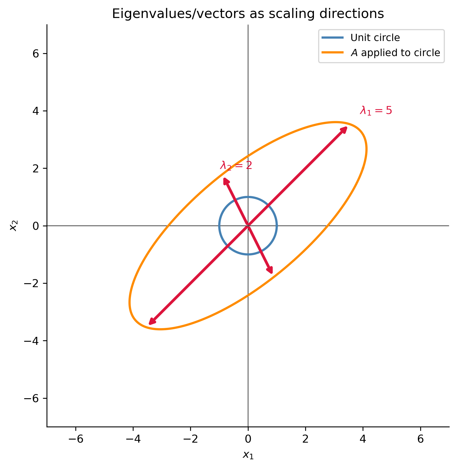
A scalar \(\lambda\) and nonzero vector \(\mathbf{v}\) satisfying \[A\mathbf{v} = \lambda\mathbf{v}\] are an eigenvalue and eigenvector of \(A\). Geometrically, \(A\) merely scales \(\mathbf{v}\) by a factor of \(\lambda\) — it does not rotate or shear it. Eigenvectors are the “special directions” that a matrix leaves invariant.

Finding eigenvalues: the equation \(A\mathbf{v}=\lambda\mathbf{v}\) has a nontrivial solution if and only if \[\det(A - \lambda I) = 0.\] This is the characteristic equation; its roots are the eigenvalues.

TipConnection to ODEs

For a constant-coefficient ODE \(x''+px'+qx=0\), the substitution \(x=e^{\lambda t}\) leads to the characteristic equation \(\lambda^2+p\lambda+q=0\). When we write the ODE as the first-order system \(\mathbf{y}'=A\mathbf{y}\), the \(\lambda\) values from the ODE characteristic equation are exactly the matrix eigenvalues of \(A\). The “eigenvalues” in Notes 4 and the matrix eigenvalues in this section are the same concept.

Computing Eigenvalues and Eigenvectors

Show the code
print("=== Example 1: 2×2 matrix ===")
A1 = np.array([[4,1],[2,3]], dtype=float)
print(f"A = {A1}")
vals, vecs = np.linalg.eig(A1)
for i, (lam, v) in enumerate(zip(vals, vecs.T)):
    print(f"  λ{i+1}={lam:.2f},  v{i+1}={v},  Av={A1@v},  λ*v={lam*v}  error={norm(A1@v-lam*v):.2e}")

print("\n=== Exact computation with SymPy ===")
A1_sym = sym.Matrix([[4,1],[2,3]])
lam = sym.Symbol('lambda')
char_eq = (A1_sym - lam*sym.eye(2)).det()
print(f"Characteristic equation: {sym.expand(char_eq)} = 0")
roots = sym.solve(char_eq, lam)
print(f"Eigenvalues: {roots}")
for root in roots:
    V = (A1_sym - root*sym.eye(2)).nullspace()
    print(f"  λ={root}: eigenvector = {V[0].T}")

print("\n=== Diagonalization: A = PDP^{-1} ===")
A1_sym2 = sym.Matrix([[4,1],[2,3]])
P, D = A1_sym2.diagonalize()
display(Math(r"P = " + sym.latex(P) + r",\quad D = " + sym.latex(D)))
print(f"Verify PDP^(-1) == A: {sym.simplify(P*D*P.inv()) == A1_sym2}")
=== Example 1: 2×2 matrix ===
A = [[4. 1.]
 [2. 3.]]
  λ1=5.00,  v1=[0.70710678 0.70710678],  Av=[3.53553391 3.53553391],  λ*v=[3.53553391 3.53553391]  error=0.00e+00
  λ2=2.00,  v2=[-0.4472136   0.89442719],  Av=[-0.89442719  1.78885438],  λ*v=[-0.89442719  1.78885438]  error=0.00e+00

=== Exact computation with SymPy ===
Characteristic equation: lambda**2 - 7*lambda + 10 = 0
Eigenvalues: [2, 5]
  λ=2: eigenvector = Matrix([[-1/2, 1]])
  λ=5: eigenvector = Matrix([[1, 1]])

=== Diagonalization: A = PDP^{-1} ===

\(\displaystyle P = \left[\begin{matrix}-1 & 1\\2 & 1\end{matrix}\right],\quad D = \left[\begin{matrix}2 & 0\\0 & 5\end{matrix}\right]\)

Verify PDP^(-1) == A: True

The Spectral Theorem for Symmetric Matrices

For symmetric matrices (\(A = A^T\)) — which arise constantly in engineering (stiffness matrices, covariance matrices, inertia tensors) — the spectral theorem guarantees:

  1. All eigenvalues are real.
  2. Eigenvectors for distinct eigenvalues are orthogonal.
  3. \(A\) is diagonalizable by an orthogonal matrix: \(A = Q\Lambda Q^T\).
Show the code
S = np.array([[4,2,0],[2,3,1],[0,1,5]], dtype=float)
vals_S, vecs_S = np.linalg.eigh(S)  # eigh guarantees real evals for symmetric
print(f"Symmetric matrix S =\n{S}\n")
print(f"Eigenvalues (all real): {np.round(vals_S, 4)}")
print(f"Orthogonality of eigenvectors (Q^T Q should be I):")
print(np.round(vecs_S.T @ vecs_S, 8))
Lambda = np.diag(vals_S)
print(f"Reconstruction S = Q*Lambda*Q^T error: {norm(vecs_S@Lambda@vecs_S.T - S):.2e}")
Symmetric matrix S =
[[4. 2. 0.]
 [2. 3. 1.]
 [0. 1. 5.]]

Eigenvalues (all real): [1.2679 4.7321 6.    ]
Orthogonality of eigenvectors (Q^T Q should be I):
[[ 1.  0. -0.]
 [ 0.  1. -0.]
 [-0. -0.  1.]]
Reconstruction S = Q*Lambda*Q^T error: 2.93e-15
Show the code
A_vis = np.array([[4,1],[2,3]], dtype=float)
vals_v, vecs_v = np.linalg.eig(A_vis)
theta = np.linspace(0, 2*np.pi, 300)
circle = np.array([np.cos(theta), np.sin(theta)])
ellipse = A_vis @ circle

fig, ax = plt.subplots(figsize=(7, 6))
ax.set_aspect('equal')
ax.axhline(0, color='k', lw=0.5); ax.axvline(0, color='k', lw=0.5)
ax.plot(*circle, color='steelblue', lw=2, label='Unit circle')
ax.plot(*ellipse, color='darkorange', lw=2, label='$A$ applied to circle')
for i, (lam, v) in enumerate(zip(vals_v, vecs_v.T)):
    ax.annotate('', xy=lam*v, xytext=[0,0],
                arrowprops=dict(arrowstyle='->', color='crimson', lw=2.5))
    ax.annotate('', xy=-lam*v, xytext=[0,0],
                arrowprops=dict(arrowstyle='->', color='crimson', lw=2.5))
    ax.text(*(lam*v*1.1), f'$\\lambda_{i+1}={lam:.0f}$', color='crimson', fontsize=10)
ax.set_xlim(-7,7); ax.set_ylim(-7,7)
ax.set_xlabel('$x_1$'); ax.set_ylabel('$x_2$')
ax.set_title('Eigenvalues/vectors as scaling directions')
ax.legend(fontsize=9)
plt.tight_layout(); plt.show()
Figure 2: Geometric effect of matrix \(A=\begin{pmatrix}4&1\\2&3\end{pmatrix}\) on the unit circle (blue). The matrix stretches the circle into an ellipse (orange). The eigenvectors (red arrows) point in the directions that are merely scaled, not rotated. The scaling factors are the eigenvalues \(\lambda_1=5\), \(\lambda_2=2\).

Part 5 — Matrix Decompositions

LU Decomposition

Every invertible matrix \(A\) can be written as \(A = PLU\), where \(P\) is a permutation matrix, \(L\) is lower-triangular with ones on the diagonal, and \(U\) is upper-triangular. This factorization is the computational engine behind solve — it reduces Gaussian elimination to two easy triangular solves.

Show the code
A_lu = np.array([[2,1,-1],[4,5,-3],[2,3,1]], dtype=float)
P_lu, L_lu, U_lu = lu(A_lu)
print(f"A =\n{A_lu}\n")
print(f"L =\n{np.round(L_lu,4)}\n")
print(f"U =\n{np.round(U_lu,4)}\n")
print(f"PLU = A: {np.allclose(P_lu@L_lu@U_lu, A_lu)}")
print(f"Solving multiple right-hand sides with LU: fast for large systems")
A =
[[ 2.  1. -1.]
 [ 4.  5. -3.]
 [ 2.  3.  1.]]

L =
[[ 1.      0.      0.    ]
 [ 0.5     1.      0.    ]
 [ 0.5    -0.3333  1.    ]]

U =
[[ 4.      5.     -3.    ]
 [ 0.     -1.5     0.5   ]
 [ 0.      0.      2.6667]]

PLU = A: True
Solving multiple right-hand sides with LU: fast for large systems

QR Decomposition

Every \(m\times n\) matrix (\(m\geq n\)) factors as \(A = QR\), where \(Q\) has orthonormal columns and \(R\) is upper-triangular. QR is numerically more stable than LU and is the basis of least-squares solvers and the standard eigenvalue algorithm (the QR algorithm).

Show the code
A_qr = np.array([[1,1,0],[1,0,1],[0,1,1],[1,1,1]], dtype=float)
Q_qr, R_qr = qr(A_qr, mode='economic')
print(f"A (4×3):\n{A_qr}\n")
print(f"Q (4×3, orthonormal columns):\n{np.round(Q_qr,4)}\n")
print(f"R (3×3, upper triangular):\n{np.round(R_qr,4)}\n")
print(f"Q^T Q = I: {np.allclose(Q_qr.T@Q_qr, np.eye(3))}")
print(f"QR = A: {np.allclose(Q_qr@R_qr, A_qr)}")
A (4×3):
[[1. 1. 0.]
 [1. 0. 1.]
 [0. 1. 1.]
 [1. 1. 1.]]

Q (4×3, orthonormal columns):
[[-0.5774  0.2582  0.6761]
 [-0.5774 -0.5164 -0.5071]
 [-0.      0.7746 -0.5071]
 [-0.5774  0.2582 -0.169 ]]

R (3×3, upper triangular):
[[-1.7321 -1.1547 -1.1547]
 [ 0.      1.291   0.5164]
 [ 0.      0.     -1.1832]]

Q^T Q = I: True
QR = A: True

Singular Value Decomposition (SVD)

The singular value decomposition is the most powerful and general matrix decomposition. Every \(m\times n\) matrix factors as: \[A = U\Sigma V^T,\] where \(U\) (\(m\times m\)) and \(V\) (\(n\times n\)) are orthogonal matrices and \(\Sigma\) is a diagonal matrix of singular values \(\sigma_1\geq\sigma_2\geq\cdots\geq 0\).

The SVD gives the definitive answers to several fundamental questions:

Question Answer via SVD
What is \(\text{rank}(A)\)? Number of nonzero \(\sigma_i\)
How ill-conditioned is \(A\)? \(\kappa(A) = \sigma_1/\sigma_r\)
Best rank-\(k\) approximation? \(A_k = \sum_{i=1}^k \sigma_i\mathbf{u}_i\mathbf{v}_i^T\)
Null space of \(A\)? Columns of \(V\) for zero \(\sigma_i\)
Pseudoinverse \(A^+\)? \(V\Sigma^+U^T\)
Show the code
A_svd = np.array([[3,2,2],[2,3,-2]], dtype=float)
U_s, sigma, VT_s = svd(A_svd)
print(f"A =\n{A_svd}\n")
print(f"Singular values σ = {sigma}")
print(f"rank(A) = {np.sum(sigma > 1e-10)}")
print(f"Condition number κ(A) = {sigma[0]/sigma[-1]:.4f}")
Sigma_full = np.zeros_like(A_svd)          # shape (2,3), matches A
np.fill_diagonal(Sigma_full, sigma)        # place singular values on diagonal
print(f"Reconstruction error ||U*Σ*V^T - A|| = {norm(U_s@Sigma_full@VT_s - A_svd):.2e}")
A =
[[ 3.  2.  2.]
 [ 2.  3. -2.]]

Singular values σ = [5. 3.]
rank(A) = 2
Condition number κ(A) = 1.6667
Reconstruction error ||U*Σ*V^T - A|| = 1.29e-15

Part 6 — Null Space, Column Space, and the Rank-Nullity Theorem

Four Fundamental Subspaces

Associated with every \(m\times n\) matrix \(A\) are four fundamental subspaces:

Subspace Definition Dimension
Column space \(\mathcal{C}(A)\) Span of columns of \(A\) \(r = \text{rank}(A)\)
Null space \(\mathcal{N}(A)\) \(\{\mathbf{x}: A\mathbf{x}=\mathbf{0}\}\) \(n-r\)
Row space \(\mathcal{C}(A^T)\) Span of rows of \(A\) \(r\)
Left null space \(\mathcal{N}(A^T)\) \(\{\mathbf{y}: A^T\mathbf{y}=\mathbf{0}\}\) \(m-r\)
ImportantRank-Nullity Theorem

\[\text{rank}(A) + \text{nullity}(A) = n.\] The number of free variables equals \(n - \text{rank}(A)\).

Show the code
B_sym = sym.Matrix([[1,2,3],[4,5,6],[7,8,9]])
print(f"Matrix A (rank-deficient):\n{B_sym}\n")
print(f"rank = {B_sym.rank()}")
print(f"Null space basis: {B_sym.nullspace()}")
print(f"Column space basis: {B_sym.columnspace()}")
print(f"Left null space: {B_sym.T.nullspace()}")
print(f"\nRank-Nullity: rank({B_sym.rank()}) + nullity({3-B_sym.rank()}) = {3}")
Matrix A (rank-deficient):
Matrix([[1, 2, 3], [4, 5, 6], [7, 8, 9]])

rank = 2
Null space basis: [Matrix([
[ 1],
[-2],
[ 1]])]
Column space basis: [Matrix([
[1],
[4],
[7]]), Matrix([
[2],
[5],
[8]])]
Left null space: [Matrix([
[ 1],
[-2],
[ 1]])]

Rank-Nullity: rank(2) + nullity(1) = 3

Part 7 — Applications in Engineering

Application 1 — Resistor Networks (Nodal Analysis)

Every electrical network satisfies Kirchhoff’s laws, which reduce to the linear system \[Y\mathbf{V} = \mathbf{I},\] where \(Y\) is the nodal admittance matrix (\(Y_{ii}\) = sum of conductances at node \(i\); \(Y_{ij}=-G_{ij}\) for \(i\neq j\)), \(\mathbf{V}\) is the vector of unknown node voltages, and \(\mathbf{I}\) is the vector of injected currents. This formulation is used in SPICE circuit simulators.

Show the code
# Network: 4 nodes (node 4 = ground = 0 V)
# Resistors: R12=2Ω, R13=4Ω, R23=3Ω, R24=1Ω, R34=5Ω
# Source: I1=5 A injected at node 1, I2=2 A injected at node 2, I3=0
G12, G13, G23, G24, G34 = 1/2, 1/4, 1/3, 1.0, 1/5

Y = np.array([
    [G12+G13,   -G12,    -G13],
    [-G12,   G12+G23+G24, -G23],
    [-G13,   -G23,    G13+G23+G34]
])
I_inj = np.array([5.0, 2.0, 0.0])  # injected currents
V_sol = solve(Y, I_inj)
print("Nodal admittance matrix Y:")
print(np.round(Y,4))
print(f"\nInjected currents I = {I_inj} A")
print(f"Node voltages: V1={V_sol[0]:.4f} V, V2={V_sol[1]:.4f} V, V3={V_sol[2]:.4f} V")
print(f"Residual ||YV - I|| = {norm(Y@V_sol - I_inj):.2e}")

# Verify by KCL at node 1: sum of outgoing currents = 5 A
I_12 = G12*(V_sol[0]-V_sol[1])
I_13 = G13*(V_sol[0]-V_sol[2])
I_14 = G13*V_sol[0]  # no direct to ground in this simplified model
print(f"\nKCL check at node 1: outgoing currents sum = {Y[0]@V_sol:.4f} A (should be 5.0)")
Nodal admittance matrix Y:
[[ 0.75   -0.5    -0.25  ]
 [-0.5     1.8333 -0.3333]
 [-0.25   -0.3333  0.7833]]

Injected currents I = [5. 2. 0.] A
Node voltages: V1=12.6250 V, V2=5.7083 V, V3=6.4583 V
Residual ||YV - I|| = 2.07e-15

KCL check at node 1: outgoing currents sum = 5.0000 A (should be 5.0)
Figure 3

Application 2 — Structural Analysis: Truss

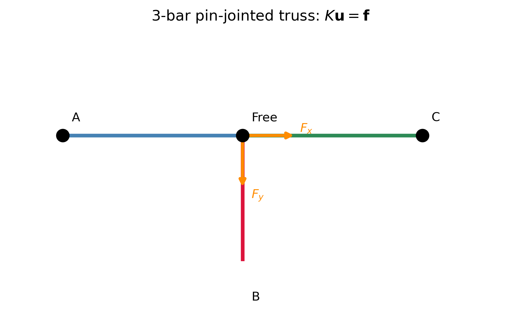
Every bar in a pin-jointed truss contributes a local stiffness matrix \(k_e = \frac{AE}{L}\begin{pmatrix}c_x^2 & c_xc_y \\ c_xc_y & c_y^2\end{pmatrix}\) where \(c_x, c_y\) are the direction cosines and \(L\) is the bar length. Summing over all bars gives the global stiffness matrix \(K\). The system \[K\mathbf{u} = \mathbf{f}\] (with boundary conditions applied) gives the displacements \(\mathbf{u}\).

Show the code
# Three bars meeting at a free node; all other nodes pinned.
# Bar 1: horizontal (angle 0°), AE=1, L=1
# Bar 2: vertical (angle 90°), AE=1, L=1
# Bar 3: diagonal (angle 45°), AE=1, L=sqrt(2)
AE_val = 100e3  # N  (typical for thin steel bar)

def bar_stiffness(AE, L, angle_deg):
    """Local stiffness contribution to 2-DOF free node"""
    th = np.radians(angle_deg)
    cx, cy = np.cos(th), np.sin(th)
    return (AE/L)*np.array([[cx**2, cx*cy],[cx*cy, cy**2]])

K_global = np.zeros((2,2))
bars_info = [(AE_val, 1.0, 0),   # horizontal
             (AE_val, 1.0, 90),  # vertical
             (AE_val, np.sqrt(2), 45)]  # diagonal

for AE_b, L_b, ang in bars_info:
    K_global += bar_stiffness(AE_b, L_b, ang)

F_applied = np.array([10e3, -20e3])  # 10 kN right, 20 kN down
u_disp = solve(K_global, F_applied)

print(f"Global stiffness matrix K [N/m]:\n{np.round(K_global,1)}\n")
print(f"Applied force F = {F_applied/1e3} kN")
print(f"Displacements u = [{u_disp[0]*1e6:.2f}, {u_disp[1]*1e6:.2f}] µm")
print(f"Residual ||Ku-F|| = {norm(K_global@u_disp - F_applied):.2e}")

# Plot truss
fig, ax = plt.subplots(figsize=(6,5))
node_free = np.array([1.0, 1.0])  # free node at center
nodes = {'A':[0,1], 'B':[1,0], 'C':[2,1], 'Free':[1,1]}
bar_conns = [('A','Free'), ('B','Free'), ('C','Free')]
colors_b = ['steelblue','crimson','seagreen']
for (n1,n2), col in zip(bar_conns, colors_b):
    p1, p2 = np.array(nodes[n1]), np.array(nodes[n2])
    ax.plot([p1[0],p2[0]], [p1[1],p2[1]], '-', color=col, lw=3)
for name, pos in nodes.items():
    ax.plot(*pos, 'ko', markersize=10, zorder=5)
    ax.text(pos[0]+0.05, pos[1]+0.08, name, fontsize=10)
ax.annotate('', xy=node_free+np.array([0.3,0]),  xytext=node_free,
            arrowprops=dict(arrowstyle='->', color='darkorange', lw=2.5))
ax.annotate('', xy=node_free+np.array([0,-0.3]), xytext=node_free,
            arrowprops=dict(arrowstyle='->', color='darkorange', lw=2.5))
ax.text(node_free[0]+0.32, node_free[1]+0.02, '$F_x$', color='darkorange')
ax.text(node_free[0]+0.05, node_free[1]-0.35, '$F_y$', color='darkorange')
ax.set_aspect('equal'); ax.set_xlim(-0.3, 2.5); ax.set_ylim(0.3, 1.6)
ax.set_title('3-bar pin-jointed truss: $K\\mathbf{u}=\\mathbf{f}$')
ax.axis('off')
plt.tight_layout(); plt.show()
Global stiffness matrix K [N/m]:
[[135355.3  35355.3]
 [ 35355.3 135355.3]]

Applied force F = [ 10. -20.] kN
Displacements u = [120710.68, -179289.32] µm
Residual ||Ku-F|| = 1.82e-12
Figure 4: Simple 3-bar planar truss. Each bar contributes a stiffness component in the direction of its axis. The global stiffness matrix is assembled by summing contributions, and \(K\mathbf{u}=\mathbf{f}\) gives the nodal displacements.

Application 3 — Least-Squares Curve Fitting

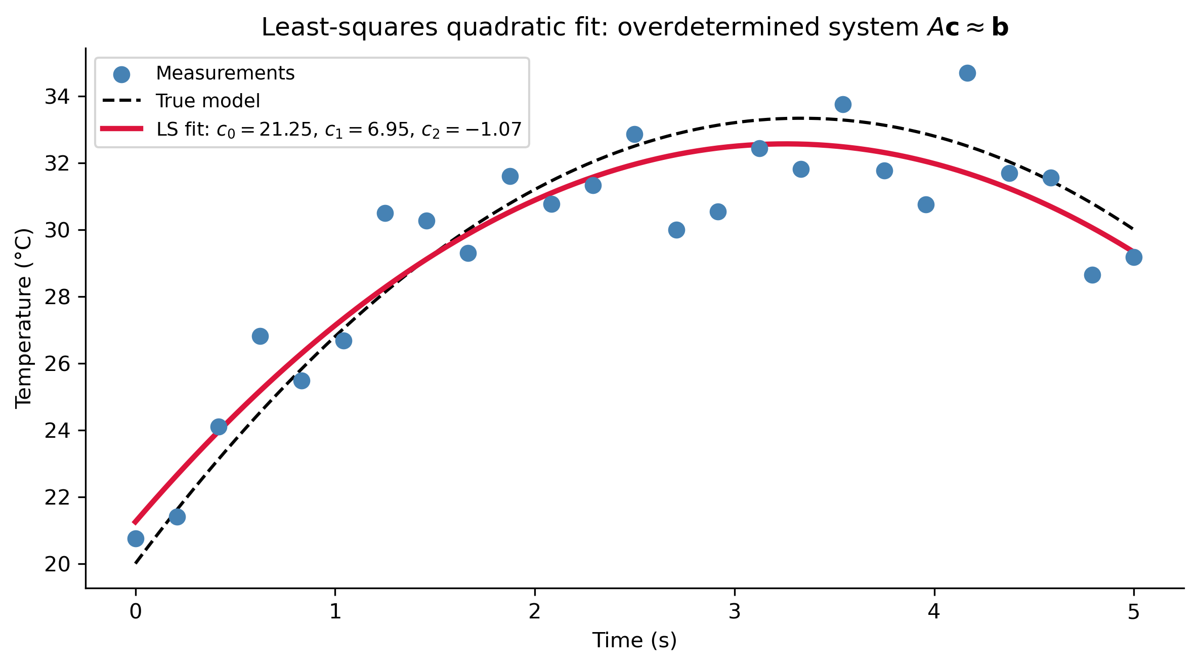
In practice, measurements give more equations than unknowns: an overdetermined system \(A\mathbf{c}\approx\mathbf{b}\) with no exact solution. The least-squares solution minimizes the residual \(\|A\mathbf{c}-\mathbf{b}\|^2\) and satisfies the normal equations \(A^TA\mathbf{c} = A^T\mathbf{b}\). This is the mathematical foundation of linear regression.

The least-squares solution is \(\mathbf{c} = (A^TA)^{-1}A^T\mathbf{b}\) (when \(A\) has full column rank), or more robustly via the pseudoinverse \(\mathbf{c} = A^+\mathbf{b}\) computed from the SVD.

Show the code
np.random.seed(42)
t_data = np.linspace(0, 5, 25)
T_true = 20 + 8*t_data - 1.2*t_data**2  # true: parabolic heating then cooling
T_meas = T_true + np.random.normal(0, 1.5, len(t_data))

# Design matrix for quadratic model
A_ls = np.column_stack([np.ones_like(t_data), t_data, t_data**2])
# Solve via normal equations
c_ls = solve(A_ls.T @ A_ls, A_ls.T @ T_meas)
# Or equivalently: c_ls, _, _, _ = lstsq(A_ls, T_meas)

t_fine = np.linspace(0, 5, 200)
T_true_fine = 20 + 8*t_fine - 1.2*t_fine**2   # true model on fine grid
A_fine = np.column_stack([np.ones_like(t_fine), t_fine, t_fine**2])
T_fit = A_fine @ c_ls

fig, ax = plt.subplots(figsize=(8, 4.5))
ax.scatter(t_data, T_meas, color='steelblue', s=50, zorder=5, label='Measurements')
ax.plot(t_fine, T_true_fine, 'k--', lw=1.5, label='True model')
ax.plot(t_fine, T_fit,  color='crimson', lw=2.5,
        label=f'LS fit: $c_0={c_ls[0]:.2f}$, $c_1={c_ls[1]:.2f}$, $c_2={c_ls[2]:.2f}$')
ax.set_xlabel('Time (s)'); ax.set_ylabel('Temperature (°C)')
ax.set_title('Least-squares quadratic fit: overdetermined system $A\\mathbf{c}\\approx\\mathbf{b}$')
ax.legend(fontsize=9)

print(f"True  coefficients: c0=20, c1=8, c2=-1.2")
print(f"Fitted coefficients: c0={c_ls[0]:.4f}, c1={c_ls[1]:.4f}, c2={c_ls[2]:.4f}")
print(f"RMS residual: {norm(A_ls@c_ls-T_meas)/np.sqrt(len(t_data)):.4f} °C")
plt.tight_layout(); plt.show()

True  coefficients: c0=20, c1=8, c2=-1.2
Fitted coefficients: c0=21.2488, c1=6.9490, c2=-1.0668
RMS residual: 1.2531 °C
Figure 5: Least-squares quadratic fit to noisy temperature vs. time data. The design matrix \(A\) has columns \([1, t, t^2]\). The normal equations \((A^TA)\mathbf{c}=A^T\mathbf{b}\) are solved for the coefficients \(\mathbf{c}=(c_0,c_1,c_2)^T\).

Application 4 — Markov Chains and Steady States

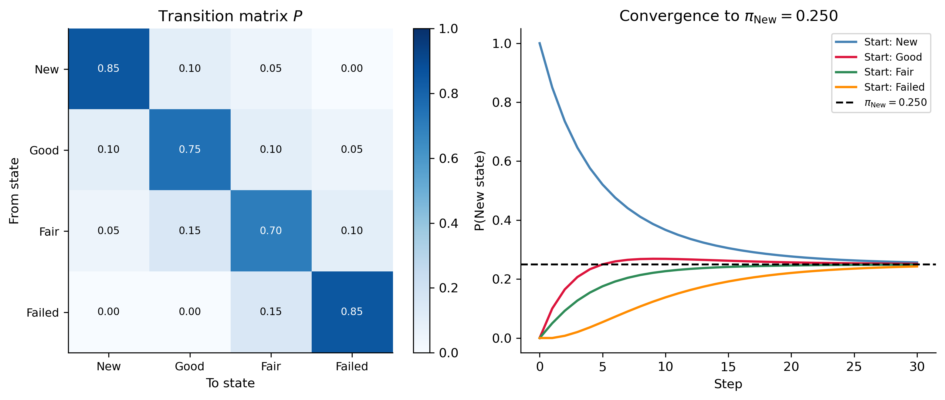
A Markov chain models a system that transitions between states with fixed probabilities. The transition matrix \(P\) (column-stochastic: columns sum to 1) satisfies \(P\boldsymbol{\pi}=\boldsymbol{\pi}\) at steady state — so \(\boldsymbol{\pi}\) is an eigenvector of \(P\) with eigenvalue 1. Finding it is a linear algebra problem.

Engineering uses: reliability analysis, queueing networks, manufacturing process control, web traffic modeling (PageRank).

Show the code
# Equipment degradation model (4 states: New, Good, Fair, Failed)
P_mc = np.array([
    [0.85, 0.10, 0.05, 0.00],   # New stays new 85%, degrades
    [0.10, 0.75, 0.10, 0.05],   # Good
    [0.05, 0.15, 0.70, 0.10],   # Fair
    [0.00, 0.00, 0.15, 0.85],   # Failed (repair brings back)
])
# Note: this is row-stochastic; P[i,j] = prob of going FROM i TO j
# Stationary: solve pi^T P = pi^T <=> P^T pi = pi
# Using: (P^T - I)pi = 0, sum(pi)=1

A_st = P_mc.T - np.eye(4)
A_st[-1,:] = 1.0
b_st = np.zeros(4); b_st[-1] = 1.0
pi_st = solve(A_st, b_st)

fig, axes = plt.subplots(1, 2, figsize=(11, 4.5))

# Heatmap
im = axes[0].imshow(P_mc, cmap='Blues', vmin=0, vmax=1)
states = ['New','Good','Fair','Failed']
axes[0].set_xticks(range(4)); axes[0].set_yticks(range(4))
axes[0].set_xticklabels(states, fontsize=9); axes[0].set_yticklabels(states, fontsize=9)
axes[0].set_xlabel('To state'); axes[0].set_ylabel('From state')
axes[0].set_title('Transition matrix $P$')
for i in range(4):
    for j in range(4):
        axes[0].text(j, i, f'{P_mc[i,j]:.2f}', ha='center', va='center',
                    fontsize=8, color='white' if P_mc[i,j]>0.5 else 'black')
plt.colorbar(im, ax=axes[0], fraction=0.046)

# Convergence from different initial states
n_steps = 30
colors_mc = ['steelblue','crimson','seagreen','darkorange']
for init_state, color in zip(range(4), colors_mc):
    x0 = np.zeros(4); x0[init_state] = 1.0
    dist = x0.copy()
    history = [dist.copy()]
    for _ in range(n_steps):
        dist = P_mc.T @ dist
        history.append(dist.copy())
    history = np.array(history)
    axes[1].plot(history[:,0], color=color, lw=1.8, label=f'Start: {states[init_state]}')
axes[1].axhline(pi_st[0], color='k', ls='--', lw=1.5, label=f'$\\pi_{{\\text{{New}}}}={pi_st[0]:.3f}$')
axes[1].set_xlabel('Step'); axes[1].set_ylabel('P(New state)')
axes[1].set_title(f'Convergence to $\\pi_{{\\text{{New}}}}={pi_st[0]:.3f}$')
axes[1].legend(fontsize=8)
print(f"Stationary distribution π = {dict(zip(states, np.round(pi_st,4)))}")
print(f"Verify P^T π = π: {np.allclose(P_mc.T @ pi_st, pi_st)}")

plt.tight_layout(); plt.show()
Stationary distribution π = {'New': np.float64(0.25), 'Good': np.float64(0.25), 'Fair': np.float64(0.25), 'Failed': np.float64(0.25)}
Verify P^T π = π: True
Figure 6: Markov chain: four states (equipment conditions: New, Good, Fair, Failed) with maintenance-driven transitions. Left: the \(4\times 4\) transition matrix visualized as a heatmap. Right: convergence of the state distribution to the stationary vector \(\boldsymbol{\pi}\) regardless of starting state.

Application 5 — Principal Component Analysis (PCA)

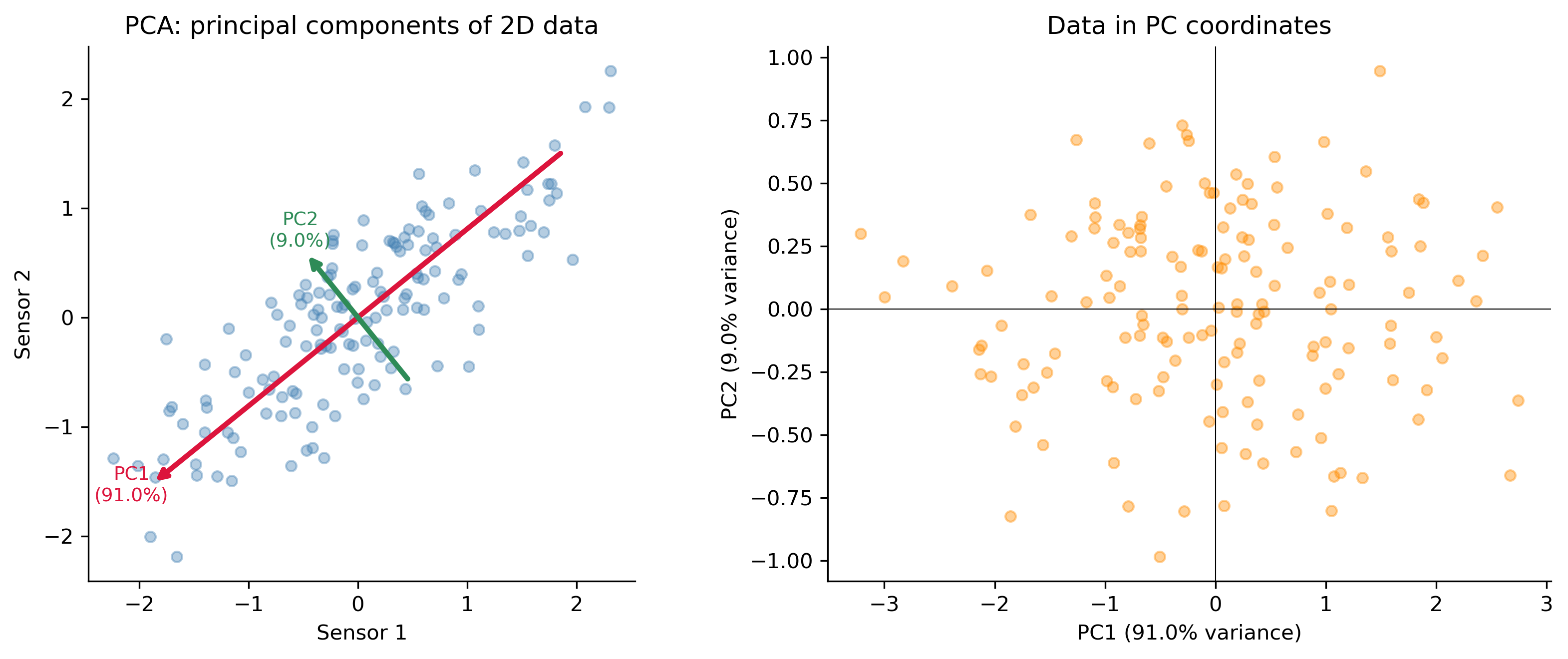
PCA finds the directions of greatest variance in a dataset. For a mean-centered data matrix \(X\) (rows = observations, columns = variables): \[X = U\Sigma V^T \quad\Longrightarrow\quad \text{principal components} = \text{columns of } V.\] The proportion of variance explained by PC \(k\) is \(\sigma_k^2/\sum_i\sigma_i^2\).

Engineering uses: dimensionality reduction, sensor fusion, structural health monitoring, signal processing, quality control.

Show the code
np.random.seed(7)
n_obs = 150
# Two correlated sensors
x1 = np.random.randn(n_obs)
x2 = 0.7*x1 + 0.5*np.random.randn(n_obs)
X_raw = np.column_stack([x1, x2])
X_c   = X_raw - X_raw.mean(axis=0)  # center

U_p, s_p, VT_p = svd(X_c, full_matrices=False)
explained = s_p**2 / np.sum(s_p**2)

fig, axes = plt.subplots(1, 2, figsize=(11, 4.5))

# Raw data + PCs
axes[0].scatter(*X_c.T, alpha=0.4, color='steelblue', s=25, label='Data')
scale = s_p / np.sqrt(n_obs-1)
for i, color in enumerate(['crimson','seagreen']):
    pc = VT_p[i,:] * scale[i]
    axes[0].annotate('', xy=pc*2, xytext=-pc*2,
                    arrowprops=dict(arrowstyle='->', color=color, lw=2.5))
    axes[0].text(*(pc*2.2), f'PC{i+1}\n({explained[i]*100:.1f}%)',
                color=color, fontsize=9, ha='center')
axes[0].set_aspect('equal')
axes[0].set_xlabel('Sensor 1'); axes[0].set_ylabel('Sensor 2')
axes[0].set_title('PCA: principal components of 2D data')

# Projected data
scores = X_c @ VT_p.T
axes[1].scatter(scores[:,0], scores[:,1], alpha=0.4, color='darkorange', s=25)
axes[1].axhline(0, color='k', lw=0.5); axes[1].axvline(0, color='k', lw=0.5)
axes[1].set_xlabel(f'PC1 ({explained[0]*100:.1f}% variance)')
axes[1].set_ylabel(f'PC2 ({explained[1]*100:.1f}% variance)')
axes[1].set_title('Data in PC coordinates')

print(f"Singular values: σ1={s_p[0]:.4f}, σ2={s_p[1]:.4f}")
print(f"Variance explained: PC1={explained[0]*100:.1f}%, PC2={explained[1]*100:.1f}%")
print(f"PC1 direction: {np.round(VT_p[0],4)}")

plt.tight_layout(); plt.show()
Singular values: σ1=14.7956, σ2=4.6493
Variance explained: PC1=91.0%, PC2=9.0%
PC1 direction: [-0.7773 -0.6291]
Figure 7: PCA on 2D correlated sensor data. Left: raw data cloud with two principal component directions (red arrows), scaled by their singular values. PC1 points along the main axis of variation; PC2 is orthogonal. Right: data projected onto the first two PCs — the scatter is maximized along PC1.

Application 6 — Low-Rank Approximation and Data Compression

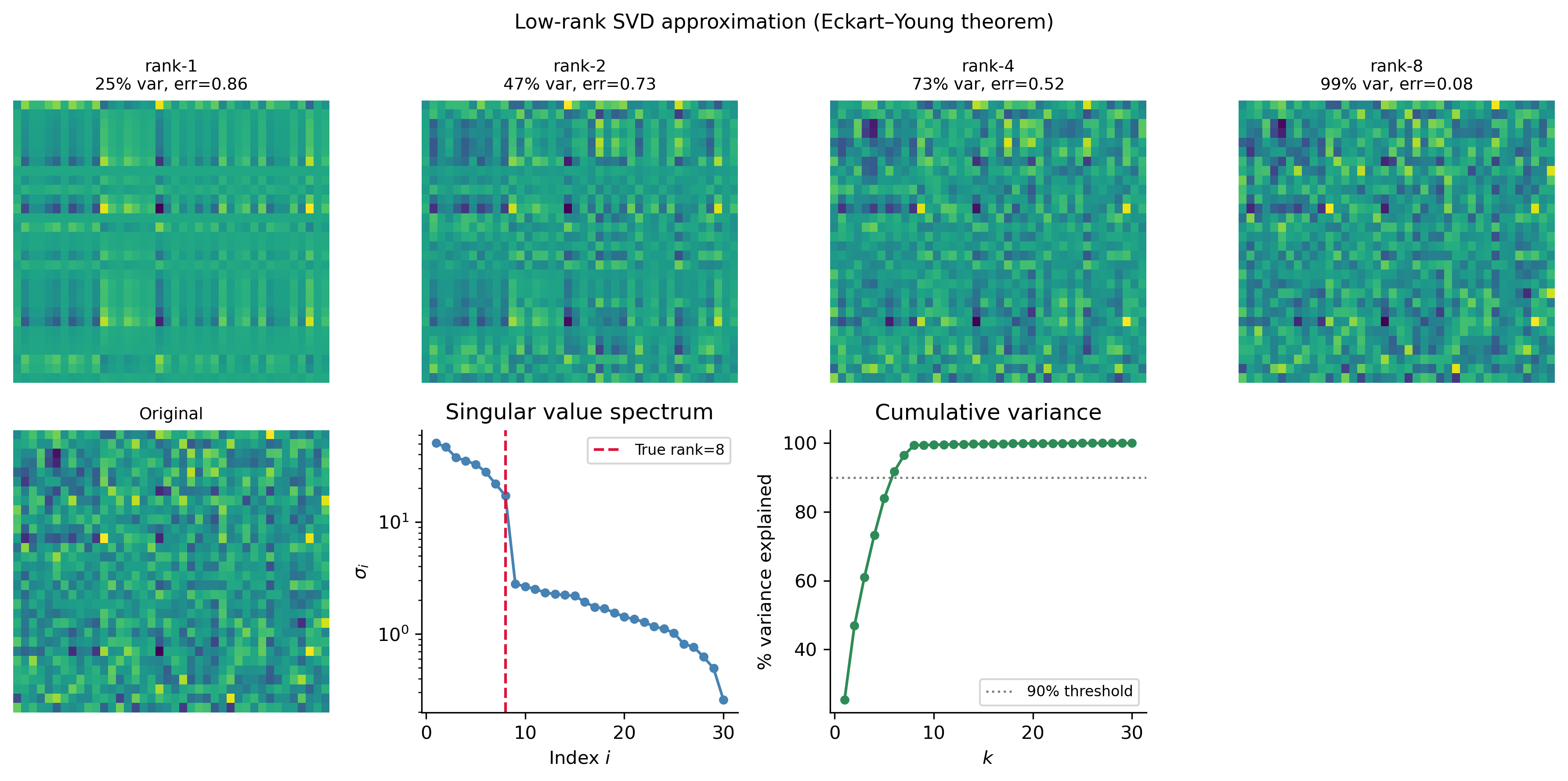
The Eckart–Young theorem states that the best rank-\(k\) approximation of \(A\) (in either the Frobenius or spectral norm) is: \[A_k = \sum_{i=1}^k \sigma_i\,\mathbf{u}_i\mathbf{v}_i^T.\] This is the foundation of image compression, collaborative filtering (Netflix-style recommendations), and model reduction in engineering simulations.

Show the code
np.random.seed(3)
m_img, n_img = 30, 40
# Create a low-rank-ish matrix (as if a simplified image)
true_rank = 8
A_img = (np.random.randn(m_img, true_rank) @ np.random.randn(true_rank, n_img)
         + 0.3*np.random.randn(m_img, n_img))
U_i, s_i, VT_i = svd(A_img)

fig, axes = plt.subplots(2, 4, figsize=(12, 6))
ranks = [1, 2, 4, true_rank]
for ax, k in zip(axes[0,:], ranks):
    A_k = U_i[:,:k] @ np.diag(s_i[:k]) @ VT_i[:k,:]
    rel_err = norm(A_img-A_k,'fro')/norm(A_img,'fro')
    var_frac = np.sum(s_i[:k]**2)/np.sum(s_i**2)
    ax.imshow(A_k, cmap='viridis', aspect='auto')
    ax.set_title(f'rank-{k}\n{var_frac*100:.0f}% var, err={rel_err:.2f}', fontsize=9)
    ax.axis('off')

# Original
axes[1,0].imshow(A_img, cmap='viridis', aspect='auto')
axes[1,0].set_title('Original', fontsize=9); axes[1,0].axis('off')

# Singular value spectrum
ax_spec = axes[1,1]
ax_spec.semilogy(range(1, len(s_i)+1), s_i, 'o-', color='steelblue', markersize=4)
ax_spec.axvline(true_rank, color='crimson', ls='--', lw=1.5, label=f'True rank={true_rank}')
ax_spec.set_xlabel('Index $i$'); ax_spec.set_ylabel('$\\sigma_i$')
ax_spec.set_title('Singular value spectrum'); ax_spec.legend(fontsize=8)

# Cumulative variance
ax_cv = axes[1,2]
cum_var = np.cumsum(s_i**2)/np.sum(s_i**2)
ax_cv.plot(range(1,len(s_i)+1), cum_var*100, 'o-', color='seagreen', markersize=4)
ax_cv.axhline(90, color='gray', ls=':', lw=1.2, label='90% threshold')
ax_cv.set_xlabel('$k$'); ax_cv.set_ylabel('% variance explained')
ax_cv.set_title('Cumulative variance'); ax_cv.legend(fontsize=8)

axes[1,3].axis('off')
plt.suptitle('Low-rank SVD approximation (Eckart–Young theorem)', fontsize=11)
plt.tight_layout(); plt.show()
Figure 8: Low-rank SVD approximation of a \(30\times 40\) test matrix (simulating a grayscale image). As the rank \(k\) increases, the reconstruction quality improves. The singular value spectrum (right) shows how rapidly the information concentrates in the first few singular values.

Part 8 — Summary: Linear Algebra with SciPy and SymPy

Quick Reference: NumPy and SciPy

import numpy as np
from scipy.linalg import solve, lu, qr, svd, norm, lstsq

A = np.array([[2.,1.,-1.],[1.,3.,2.],[3.,-1.,1.]])
b = np.array([8., 14., 2.])

# Solving
x = solve(A, b)                           # exact solution
x_ls, _, _, _ = lstsq(A[:2,:], b[:2])    # least squares

# Factorizations
P, L, U     = lu(A)
Q, R        = qr(A)
U_s, s, VT  = svd(A)

# Eigenvalues
vals, vecs  = np.linalg.eig(A)           # general
vals_sym    = np.linalg.eigh(A)[0]       # symmetric (real, sorted)

# Matrix properties
print(f"det={np.linalg.det(A):.2f}, rank={np.linalg.matrix_rank(A)}")
print(f"cond={np.linalg.cond(A):.4f}, trace={np.trace(A):.2f}")
print(f"norm (Frobenius)={norm(A,'fro'):.4f}, norm (2)={norm(A,2):.4f}")
det=25.00, rank=3
cond=2.2030, trace=6.00
norm (Frobenius)=5.5678, norm (2)=4.1175

Quick Reference: SymPy

import sympy as sym

A_s = sym.Matrix([[4,1],[2,3]])

print("Determinant:", A_s.det())
print("Inverse:\n", A_s.inv())
print("Eigenvalues:", A_s.eigenvals())
print("Eigenvectors:")
for val, mult, vecs in A_s.eigenvects():
    print(f"  λ={val}, multiplicity={mult}, v={vecs}")

rref_A, pivots = A_s.rref()
print("RREF:", rref_A)
P_d, D_d = A_s.diagonalize()
print(f"Diagonalization: P={P_d}, D={D_d}")
null_A = sym.Matrix([[1,2,3],[4,5,6],[7,8,9]]).nullspace()
print(f"Null space: {null_A}")
Determinant: 10
Inverse:
 Matrix([[3/10, -1/10], [-1/5, 2/5]])
Eigenvalues: {5: 1, 2: 1}
Eigenvectors:
  λ=2, multiplicity=1, v=[Matrix([
[-1/2],
[   1]])]
  λ=5, multiplicity=1, v=[Matrix([
[1],
[1]])]
RREF: Matrix([[1, 0], [0, 1]])
Diagonalization: P=Matrix([[-1, 1], [2, 1]]), D=Matrix([[2, 0], [0, 5]])
Null space: [Matrix([
[ 1],
[-2],
[ 1]])]

Summary of Key Concepts

Concept Notation Significance
Dot product \(\mathbf{u}\cdot\mathbf{v}\) Geometry, projections, orthogonality
Matrix-vector product \(A\mathbf{x}\) Linear transformation
Determinant \(\det(A)\) Invertibility, volume scaling
Rank \(\text{rank}(A)\) Dimension of column space
Null space \(\mathcal{N}(A)\) Solution space of \(A\mathbf{x}=\mathbf{0}\)
Eigenvalue/vector \(A\mathbf{v}=\lambda\mathbf{v}\) Invariant directions and scaling
LU decomposition \(A=PLU\) Solving linear systems efficiently
QR decomposition \(A=QR\) Least squares, numerically stable
SVD \(A=U\Sigma V^T\) Best low-rank approx, condition number
Condition number \(\kappa=\sigma_1/\sigma_r\) Numerical sensitivity
Least squares \(\min\|A\mathbf{c}-\mathbf{b}\|\) Overdetermined systems, regression

Relevant Videos

Modeling with Matrices and Vectors:

References

Show the code
import sys
print("Python:", sys.version)
print('\n'.join(f'{m.__name__}=={m.__version__}' for m in globals().values() if getattr(m,'__version__',None)))
Python: 3.14.4 | packaged by conda-forge | (main, Apr  8 2026, 02:33:53) [Clang 20.1.8 ]
numpy==2.4.3
sympy==1.14.0
matplotlib==3.10.8

Reuse

CC BY-NC-SA 4.0