RLC Circuits, Filters, and the DC Motor

Electrical and Electro-Mechanical Applications of ODEs

Show the code

import numpy as np
import sympy as sym
import matplotlib as mpl
import matplotlib.pyplot as plt
from scipy.integrate import solve_ivp
from IPython.display import Math, display
mpl.rcParams['figure.dpi'] = 150
mpl.rcParams['axes.spines.top'] = False
mpl.rcParams['axes.spines.right'] = False

Second-order linear ODEs with constant coefficients — the subject of Notes 4 and Topics 5 — are not merely abstract mathematics. They are the governing equations of an enormous class of electrical and electro-mechanical devices that underpin modern technology: amplifiers, filters, oscillators, radio receivers, and electric motors. This section develops three progressively richer applications, each of which illuminates a different aspect of the ODE theory.

The RC low-pass filter — a first-order linear ODE whose frequency-dependent solution is the foundation of signal processing.
The series RLC circuit — the electrical twin of the damped oscillator, with free response, driven response, impedance, the quality factor $Q$, and the AM radio receiver as a capstone application.
The DC motor — an electro-mechanical system governed by a coupled first-order system that reduces to a second-order ODE, bridging Notes 4 and the Chapter 3 systems material.

Part 1 — The RC Low-Pass Filter

Circuit Equation

An RC circuit consists of a resistor $R$ and capacitor $C$ in series. When driven by an input voltage $V_{in}(t)$, Kirchhoff’s voltage law gives: \[ V_R + V_C = V_{in}(t), \] where $V_R = RI = RC\,V_C'$ (using $I = C\,V_C'$). Substituting: \[ \boxed{RC\,V_C' + V_C = V_{in}(t).} \tag{RC} \] This is a first-order linear ODE — the integrating-factor equation from Notes 2, with $p = 1/(RC)$ and forcing $V_{in}(t)/(RC)$.

The quantity $\tau = RC$ is the time constant of the circuit. It has units of seconds (ohms $\times$ farads $= $ s) and governs how quickly the capacitor charges or discharges.

Step Response

With $V_{in}(t) = E_0$ (a battery switched on at $t=0$) and $V_C(0) = 0$: \[ V_C(t) = E_0\!\left(1 - e^{-t/\tau}\right). \] The capacitor charges toward $E_0$, reaching $63.2\%$ of $E_0$ at $t = \tau$ and essentially fully charged ($>99\%$) at $t = 5\tau$.

Frequency Response — The Low-Pass Filter

When the input is a sinusoid $V_{in}(t) = V_0\cos(\omega t)$, the steady-state output (particular solution) is: \[ V_C(t) = \frac{V_0}{\sqrt{1 + (\omega\tau)^2}}\cos(\omega t - \phi), \qquad \phi = \arctan(\omega\tau). \] The amplitude ratio (or transfer function magnitude) is: \[ \boxed{|H(\omega)| = \frac{|V_C|}{|V_{in}|} = \frac{1}{\sqrt{1 + (\omega\tau)^2}}.} \]

This function is close to 1 for low frequencies ($\omega\tau \ll 1$) and falls off for high frequencies ($\omega\tau \gg 1$) — the circuit passes low frequencies and attenuates high frequencies. This is a low-pass filter.

The cut-off frequency is $\omega_c = 1/\tau = 1/(RC)$, where $|H| = 1/\sqrt{2} \approx 0.707$ (a $3\,\text{dB}$ reduction in power).

Decibels

Signal engineers express amplitude ratios in decibels: $|H|_{\text{dB}} = 20\log_{10}|H|$. At the cut-off frequency: $20\log_{10}(1/\sqrt{2}) \approx -3\,\text{dB}$. Above $\omega_c$ the RC filter rolls off at $-20\,\text{dB/decade}$ (amplitude drops by a factor of 10 every time $\omega$ increases by a factor of 10).

Show the code

R_val  = 1e3     # 1 kΩ
C_val  = 1e-6    # 1 μF
tau    = R_val * C_val   # 1 ms
fc     = 1/(2*np.pi*tau) # 159 Hz
E0     = 5.0

fig, axes = plt.subplots(1, 2, figsize=(11, 4.5))

# ── Step response ────────────────────────────────────────────
t_step = np.linspace(0, 6*tau, 400)
V_step = E0 * (1 - np.exp(-t_step/tau))
axes[0].plot(t_step*1e3, V_step, color='steelblue', lw=2.5)
axes[0].axhline(E0, color='k', ls='--', lw=1, label=f'$E_0={E0}$ V')
axes[0].axvline(tau*1e3, color='crimson', ls=':', lw=1.5,
                label=f'$\\tau={tau*1e3:.0f}$ ms ($V_C=0.632E_0$)')
axes[0].plot(tau*1e3, E0*(1-1/np.e), 'ro', markersize=7, zorder=5)
axes[0].set_xlabel('Time (ms)'); axes[0].set_ylabel('$V_C(t)$ (V)')
axes[0].set_title('Step response ($V_{in}=5$ V, $V_C(0)=0$)')
axes[0].legend(fontsize=8.5); axes[0].set_ylim(0, 5.5)

# ── Bode magnitude plot ──────────────────────────────────────
f_arr = np.logspace(1, 5, 500)  # 10 Hz to 100 kHz
omega_arr = 2*np.pi*f_arr
H_mag  = 1.0/np.sqrt(1 + (tau*omega_arr)**2)
H_dB   = 20*np.log10(H_mag)
# -20 dB/decade asymptote
H_asymp = np.where(f_arr < fc, np.zeros_like(f_arr),
                   20*np.log10(fc/f_arr))

axes[1].semilogx(f_arr, H_dB, color='steelblue', lw=2.5, label='$|H(f)|$ (dB)')
axes[1].semilogx(f_arr, H_asymp, color='crimson', lw=1.5, ls='--',
                 label='$-20$ dB/decade asymptote')
axes[1].axvline(fc, color='darkorange', ls=':', lw=1.5,
                label=f'Cut-off $f_c={fc:.0f}$ Hz ($-3$ dB)')
axes[1].axhline(-3, color='darkorange', ls=':', lw=1)
axes[1].set_xlabel('Frequency (Hz)'); axes[1].set_ylabel('$|H|$ (dB)')
axes[1].set_title('Bode magnitude plot (log frequency)')
axes[1].legend(fontsize=8); axes[1].set_ylim(-60, 5)
axes[1].grid(True, which='both', alpha=0.3)

plt.suptitle(f'RC Low-Pass Filter ($R={R_val/1e3:.0f}\\,\\mathrm{{k}}\\Omega$, '
             f'$C={C_val*1e6:.0f}\\,\\mu\\mathrm{{F}}$, '
             f'$\\tau={tau*1e3:.0f}\\,\\mathrm{{ms}}$)', fontsize=11)
plt.tight_layout()
plt.show()

Figure 1: RC low-pass filter ($R=1\,\text{k}\Omega$, $C=1\,\mu\text{F}$, $\tau=1\,\text{ms}$, $f_c=159\,\text{Hz}$). Left: step response — the capacitor charges toward $E_0=5\,\text{V}$ with time constant $\tau$. Right: Bode magnitude plot — the filter passes low frequencies and attenuates high frequencies, rolling off at $-20\,\text{dB/decade}$ above $f_c$.

Part 2 — The Series RLC Circuit

Circuit Equation

A series RLC circuit contains a resistor $R$, inductor $L$, and capacitor $C$ in series, driven by voltage $E(t)$. Kirchhoff’s voltage law gives $V_R + V_L + V_C = E(t)$, i.e., \[ RI + L\,\frac{dI}{dt} + \frac{Q}{C} = E(t). \] Since $I = Q'$ (current is rate of change of charge): \[ \boxed{L\,Q'' + R\,Q' + \frac{Q}{C} = E(t).} \tag{RLC} \] This is a second-order linear ODE with constant coefficients — structurally identical to the forced damped oscillator. Dividing by $L$: \[ Q'' + 2\alpha\,Q' + \omega_0^2\,Q = \frac{E(t)}{L}, \] where the damping coefficient $\alpha = R/(2L)$ and the resonant frequency $\omega_0 = 1/\sqrt{LC}$.

The Mechanical–Electrical Correspondence

Mechanical	Symbol	Electrical	Symbol
Mass	$m$	Inductance	$L$
Damping	$\gamma$	Resistance	$R$
Spring constant	$k$	$1/C$	$1/C$
Displacement	$x$	Charge	$Q$
Velocity	$x'$	Current	$I$

Every result from the spring–mass analysis in Topics 5 carries over directly.

Free Response: Three Damping Regimes

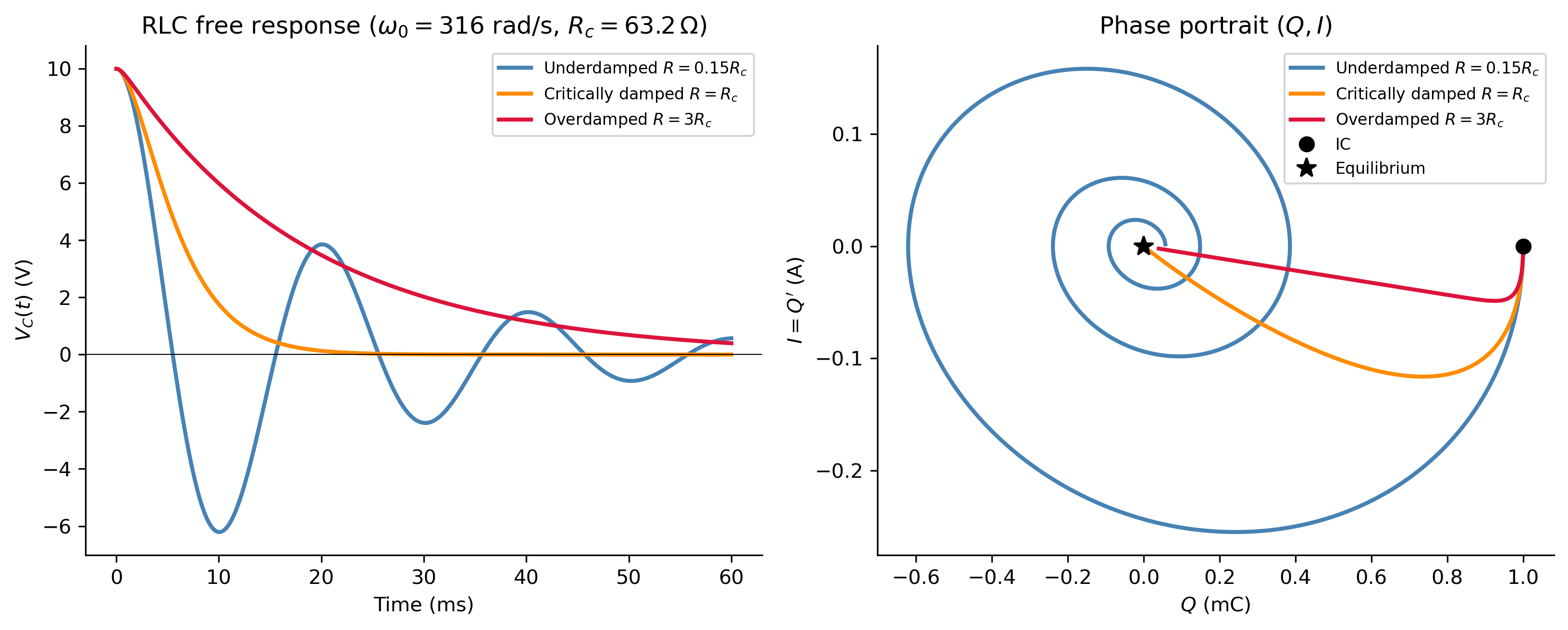
With $E(t)=0$ and initial charge $Q_0 = CV_0$ (capacitor pre-charged to voltage $V_0$), $I(0)=0$:

Underdamped ($R < 2\sqrt{L/C}$): oscillatory discharge at damped frequency $\omega_d = \sqrt{\omega_0^2 - \alpha^2}$: \[ Q(t) = Q_0\,e^{-\alpha t}\!\left(\cos\omega_d t + \frac{\alpha}{\omega_d}\sin\omega_d t\right). \]

Critically damped ($R = 2\sqrt{L/C}$): fastest non-oscillatory discharge $(C_1 + C_2 t)e^{-\alpha t}$.

Overdamped ($R > 2\sqrt{L/C}$): slow exponential discharge $C_1 e^{\lambda_1 t} + C_2 e^{\lambda_2 t}$.

Show the code

L_val = 0.1     # H
C_val = 1e-4    # 100 μF
V0    = 10.0    # initial voltage
Q0    = C_val * V0

omega0 = 1/np.sqrt(L_val*C_val)  # 316.2 rad/s
R_crit = 2*np.sqrt(L_val/C_val)  # critical resistance

R_cases = [
    (R_crit*0.15, 'steelblue',  'Underdamped $R=0.15R_c$'),
    (R_crit,      'darkorange', 'Critically damped $R=R_c$'),
    (R_crit*3.0,  'crimson',    'Overdamped $R=3R_c$'),
]

fig, axes = plt.subplots(1, 2, figsize=(11, 4.5))
t_plot = np.linspace(0, 0.06, 1000)

for R_val, color, lbl in R_cases:
    alpha = R_val/(2*L_val)
    def rlc_free(t, y, a=alpha):
        return [y[1], -2*a*y[1] - omega0**2*y[0]]
    sol = solve_ivp(rlc_free, (0, 0.06), [Q0, 0.0], t_eval=t_plot, max_step=5e-5)
    Vc = sol.y[0] / C_val  # voltage across capacitor
    axes[0].plot(sol.t*1e3, Vc, color=color, lw=2, label=lbl)
    axes[1].plot(sol.y[0]*1e3, sol.y[1], color=color, lw=2, label=lbl)

axes[0].axhline(0, color='k', lw=0.5)
axes[0].set_xlabel('Time (ms)'); axes[0].set_ylabel('$V_C(t)$ (V)')
axes[0].set_title(f'RLC free response ($\\omega_0={omega0:.0f}$ rad/s, $R_c={R_crit:.1f}\\,\\Omega$)')
axes[0].legend(fontsize=8)

axes[1].plot(Q0*1e3, 0, 'ko', markersize=7, label='IC', zorder=5)
axes[1].plot(0, 0, 'k*', markersize=10, label='Equilibrium', zorder=5)
axes[1].set_xlabel('$Q$ (mC)'); axes[1].set_ylabel('$I = Q\'$ (A)')
axes[1].set_title('Phase portrait $(Q, I)$')
axes[1].legend(fontsize=8)

plt.tight_layout()
plt.show()

Figure 2: RLC free response ($L=0.1\,\text{H}$, $C=100\,\mu\text{F}$, $V_0=10\,\text{V}$). Left: capacitor voltage $V_C=Q/C$ for three damping regimes. The underdamped circuit oscillates like a decaying spring. Right: phase portrait $(Q, I)$ — the underdamped case spirals inward; the overdamped case decays without orbiting.

Driven Response: Impedance and the Quality Factor

With sinusoidal driving $E(t) = E_0\cos(\omega t)$, the steady-state current is $I(t) = I_0\cos(\omega t - \phi)$ where the amplitude is determined by the electrical impedance:

\[ |Z(\omega)| = \sqrt{R^2 + \left(\omega L - \frac{1}{\omega C}\right)^2}. \]

The three contributions to impedance are:

Element	Impedance	Behavior
Resistor	$Z_R = R$	Constant — dissipates energy
Inductor	$Z_L = \omega L$	Increases with $\omega$ — opposes current change
Capacitor	$Z_C = 1/(\omega C)$	Decreases with $\omega$ — opposes voltage change

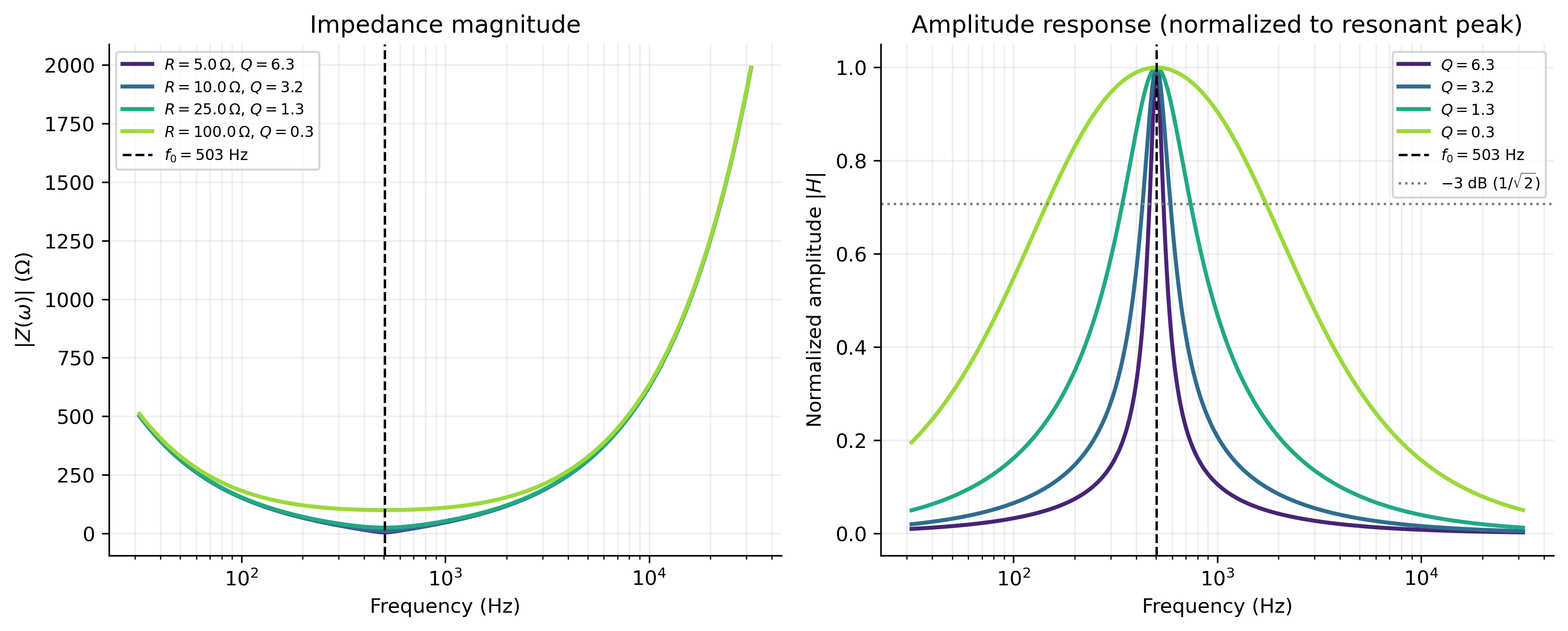
At resonance $\omega = \omega_0 = 1/\sqrt{LC}$, the inductive and capacitive impedances cancel exactly ($\omega_0 L = 1/(\omega_0 C)$), leaving only the resistance: \[ |Z(\omega_0)| = R \quad\longrightarrow\quad I_{\max} = \frac{E_0}{R}. \]

The Quality Factor $Q$

The quality factor (or $Q$-factor) characterizes how sharp the resonance peak is:

\[ \boxed{Q = \frac{\omega_0 L}{R} = \frac{1}{\omega_0 CR} = \frac{\omega_0}{2\alpha} = \frac{f_0}{\Delta f},} \]

where $\Delta f$ is the bandwidth — the frequency range over which the power is within $3\,\text{dB}$ of the peak. A high-$Q$ circuit has a sharp, narrow resonance; a low-$Q$ circuit has a broad, flat response.

$Q$ value	Resonance character	Damping regime
$Q < 1/2$	Overdamped (no resonance peak)	Over
$Q = 1/\sqrt{2}$	Maximally flat (Butterworth)	Critical–ish
$Q > 1/2$	Resonance peak appears	Under
$Q \gg 1$	Very sharp, highly selective	Lightly damped

Show the code

L_v  = 10e-3   # 10 mH
C_v  = 10e-6   # 10 μF
omega0_v = 1/np.sqrt(L_v*C_v)

R_vals = [5.0, 10.0, 25.0, 100.0]
Q_vals_computed = [omega0_v*L_v/R for R in R_vals]
colors_r = plt.cm.viridis(np.linspace(0.1, 0.85, len(R_vals)))

f_arr   = np.logspace(1.5, 4.5, 1000)
omega_r = 2*np.pi*f_arr

fig, axes = plt.subplots(1, 2, figsize=(11, 4.5))

for R, Qc, color in zip(R_vals, Q_vals_computed, colors_r):
    Z  = np.sqrt(R**2 + (omega_r*L_v - 1/(omega_r*C_v))**2)
    H  = R/Z   # normalized: current amplitude / max current
    axes[0].semilogx(f_arr, Z, color=color, lw=2, label=f'$R={R}\\,\\Omega$, $Q={Qc:.1f}$')
    axes[1].semilogx(f_arr, H, color=color, lw=2, label=f'$Q={Qc:.1f}$')

f0_v = omega0_v/(2*np.pi)
for ax in axes:
    ax.axvline(f0_v, color='k', ls='--', lw=1.2, label=f'$f_0={f0_v:.0f}$ Hz')
    ax.set_xlabel('Frequency (Hz)')
    ax.grid(True, which='both', alpha=0.2)

axes[0].set_ylabel('$|Z(\\omega)|$ ($\\Omega$)')
axes[0].set_title('Impedance magnitude')
axes[0].legend(fontsize=7.5)

axes[1].axhline(1/np.sqrt(2), color='gray', ls=':', lw=1.2, label='$-3$ dB ($1/\\sqrt{2}$)')
axes[1].set_ylabel('Normalized amplitude $|H|$')
axes[1].set_title('Amplitude response (normalized to resonant peak)')
axes[1].legend(fontsize=7.5)

plt.tight_layout()
plt.show()

Figure 3: Series RLC driven response ($L=10\,\text{mH}$, $C=10\,\mu\text{F}$, $\omega_0\approx 3162\,\text{rad/s}$, $f_0\approx 503\,\text{Hz}$). Left: impedance $|Z(\omega)|$ vs. frequency for four values of $R$. The minimum impedance at resonance equals $R$. Right: normalized amplitude response $|H(\omega)| = R/|Z(\omega)|$ — the curves are labeled by their $Q$ factor. Higher $Q$ gives a sharper, taller peak.

Application: The AM Radio Receiver

The classic application of RLC resonance is the AM radio receiver.

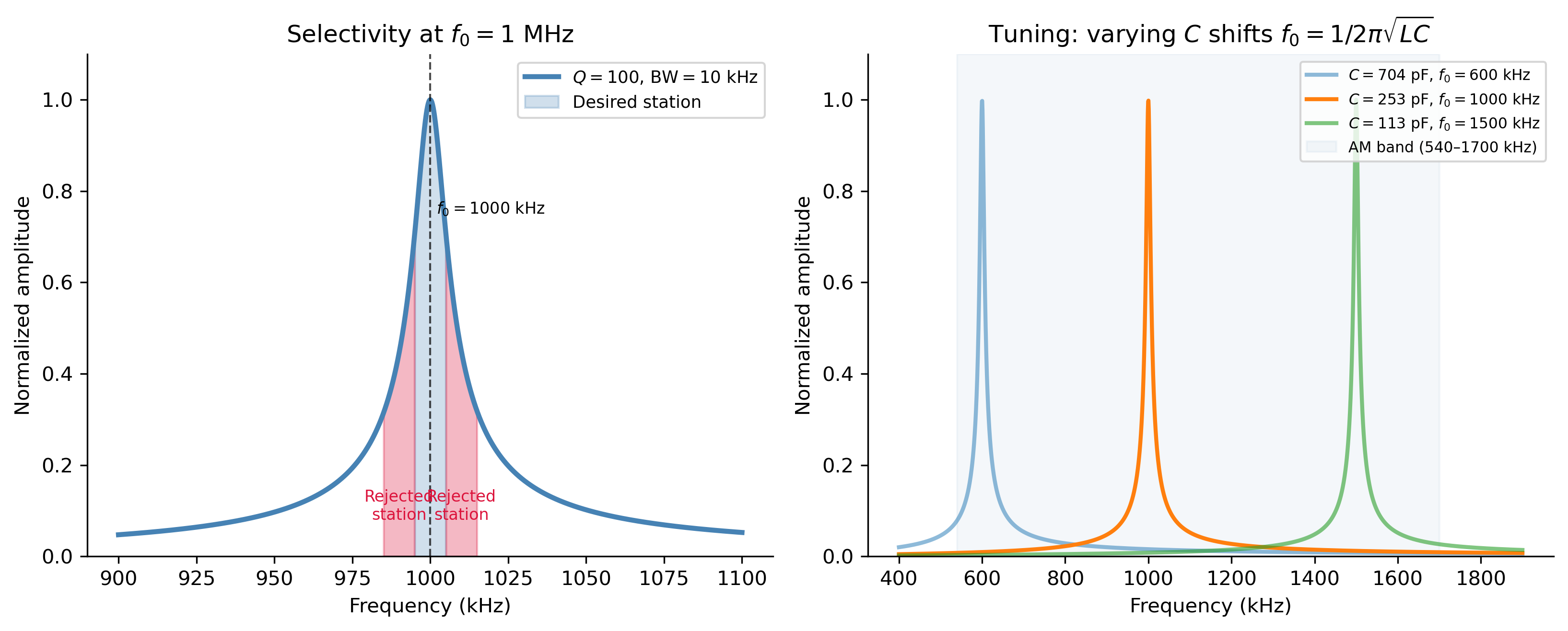
How AM radio works. The AM band spans 540–1700 kHz with stations spaced 10 kHz apart. Each station broadcasts at a specific carrier frequency $f_s$. At the antenna, all stations arrive simultaneously as a superposition of sinusoidal signals. The receiver must select one station and reject all others.

The tuning circuit. A series (or parallel) RLC circuit with variable capacitor $C$ acts as a bandpass filter. By adjusting $C$, the resonant frequency \[ f_0 = \frac{1}{2\pi\sqrt{LC}} \] is tuned to match the desired station $f_s = f_0$. At resonance the circuit responds strongly to the signal at $f_s$ and attenuates all other frequencies.

Selectivity and $Q$. The bandwidth of the tuning circuit must be: - Wide enough to pass the audio sidebands ($\pm 5$ kHz around the carrier). - Narrow enough to reject adjacent stations (spaced 10 kHz away).

This requires $Q \approx f_0 / \Delta f \approx 1000\,\text{kHz} / 10\,\text{kHz} = 100$.

Show the code

L_am  = 100e-6   # 100 μH
R_am  = 6.28     # Ω  => Q = omega0*L/R = 100 at 1 MHz
C_am  = 253.3e-12  # 253.3 pF => f0 = 1 MHz

fig, axes = plt.subplots(1, 2, figsize=(11, 4.5))

# ── Selectivity at f0=1 MHz ──────────────────────────────────
f_arr  = np.linspace(900e3, 1100e3, 2000)
omega_ = 2*np.pi*f_arr
Z_am   = np.sqrt(R_am**2 + (omega_*L_am - 1/(omega_*C_am))**2)
H_am   = R_am/Z_am

f0_am  = 1/(2*np.pi*np.sqrt(L_am*C_am))
Q_am   = f0_am*L_am*2*np.pi/R_am
BW_am  = f0_am/Q_am

axes[0].plot(f_arr/1e3, H_am, color='steelblue', lw=2.5, label=f'$Q={Q_am:.0f}$, BW$={BW_am/1e3:.0f}$ kHz')
axes[0].axvline(f0_am/1e3, color='k', ls='--', lw=1, alpha=0.7)
# Desired station passband
mask_pass = np.abs(f_arr - f0_am) < BW_am/2
axes[0].fill_between(f_arr[mask_pass]/1e3, 0, H_am[mask_pass],
                     alpha=0.25, color='steelblue', label='Desired station')
# Adjacent stations
for f_adj in [990e3, 1010e3]:
    mask_adj = (np.abs(f_arr - f_adj) < 5e3)
    axes[0].fill_between(f_arr[mask_adj]/1e3, 0, H_am[mask_adj],
                         alpha=0.3, color='crimson')
axes[0].annotate('Rejected\nstation', xy=(990, 0.08), fontsize=8, ha='center', color='crimson')
axes[0].annotate('Rejected\nstation', xy=(1010, 0.08), fontsize=8, ha='center', color='crimson')
axes[0].annotate(f'$f_0={f0_am/1e3:.0f}$ kHz', xy=(f0_am/1e3+2, 0.75), fontsize=8)
axes[0].set_xlabel('Frequency (kHz)'); axes[0].set_ylabel('Normalized amplitude')
axes[0].set_title('Selectivity at $f_0=1$ MHz')
axes[0].legend(fontsize=8.5); axes[0].set_ylim(0, 1.1)

# ── Tuning by varying C ──────────────────────────────────────
f_tune = np.linspace(540e3, 1700e3, 200)  # AM band
C_tune = 1/(L_am*(2*np.pi*f_tune)**2)    # capacitance needed for each f0
f_sweep = np.linspace(400e3, 1900e3, 2000)
for f_target, alpha_val in zip([600e3, 1000e3, 1500e3], [0.5, 1.0, 0.6]):
    C_t = 1/(L_am*(2*np.pi*f_target)**2)
    omega_s = 2*np.pi*f_sweep
    Z_t = np.sqrt(R_am**2 + (omega_s*L_am - 1/(omega_s*C_t))**2)
    H_t = R_am/Z_t
    lbl = f'$C={C_t*1e12:.0f}$ pF, $f_0={f_target/1e3:.0f}$ kHz'
    axes[1].plot(f_sweep/1e3, H_t, lw=2, label=lbl, alpha=alpha_val if alpha_val<1 else 1.0)

axes[1].axvspan(540, 1700, alpha=0.06, color='steelblue', label='AM band (540–1700 kHz)')
axes[1].set_xlabel('Frequency (kHz)'); axes[1].set_ylabel('Normalized amplitude')
axes[1].set_title('Tuning: varying $C$ shifts $f_0 = 1/2\\pi\\sqrt{LC}$')
axes[1].legend(fontsize=7.5); axes[1].set_ylim(0, 1.1)

plt.tight_layout()
plt.show()

Figure 4: AM radio tuning circuit ($L=100\,\mu\text{H}$, $R=6.28\,\Omega$, $Q=100$, $f_0=1\,\text{MHz}$). Left: amplitude response centered at $f_0=1\,\text{MHz}$ with bandwidth $\Delta f = 10\,\text{kHz}$ — the circuit passes the desired station (shaded blue) and rejects neighboring stations (shaded red). Right: how varying $C$ shifts the resonant frequency to tune across the AM band (540–1700 kHz).

From ODE to Engineering Design

The AM tuning circuit is the ODE amplitude response function $G(\Omega)$ applied as an engineering specification: - Center frequency $f_0 = 1/(2\pi\sqrt{LC})$ sets which station is received. - Bandwidth $\Delta f = R/(2\pi L)$ sets selectivity. - Q factor $Q = f_0/\Delta f = \omega_0 L/R$ is the single dimensionless parameter that characterizes the tradeoff between selectivity and audio fidelity. Every AM, FM, and digital radio ever built relies on this mathematics.

Part 3 — The DC Motor

Physical Setup

A DC motor converts electrical energy into mechanical rotation. The key components are:

Armature circuit: a coil of wire (resistance $R_a$, inductance $L_a$) rotating in a magnetic field. When current $I(t)$ flows, it produces a torque $T_m = K_T I$ ($K_T$ = torque constant).
Back-EMF: as the coil rotates at angular velocity $\omega(t)$, it generates a back-electromotive force $e_b = K_b\omega$ ($K_b$ = back-EMF constant) that opposes the applied voltage.
Mechanical load: the rotating shaft has moment of inertia $J$ and experiences viscous friction torque $b\omega$ (damping coefficient $b$).

Governing ODEs

Applying Kirchhoff’s voltage law to the armature circuit: \[ L_a\,I' + R_a\,I + K_b\,\omega = V(t). \tag{E} \] Applying Newton’s second law for rotation: \[ J\,\omega' + b\,\omega = K_T\,I. \tag{M} \] This is a coupled system of two first-order linear ODEs — a preview of the Chapter 3 systems material.

Reduction to a Second-Order ODE

We can eliminate $I$ to obtain a single second-order ODE for $\omega$. From (M): $I = (J\omega' + b\omega)/K_T$. Differentiating and substituting into (E): \[ \frac{L_a}{K_T}(J\omega'' + b\omega') + \frac{R_a}{K_T}(J\omega' + b\omega) + K_b\omega = V(t). \] Multiplying by $K_T$ and rearranging: \[ \boxed{(JL_a)\,\omega'' + (JR_a + bL_a)\,\omega' + (bR_a + K_bK_T)\,\omega = K_T\,V(t).} \tag{Motor} \] This has the same form as the forced damped oscillator! The eigenvalues of the characteristic equation determine whether the motor oscillates (unusual) or converges smoothly to its steady-state speed.

Steady-State Speed

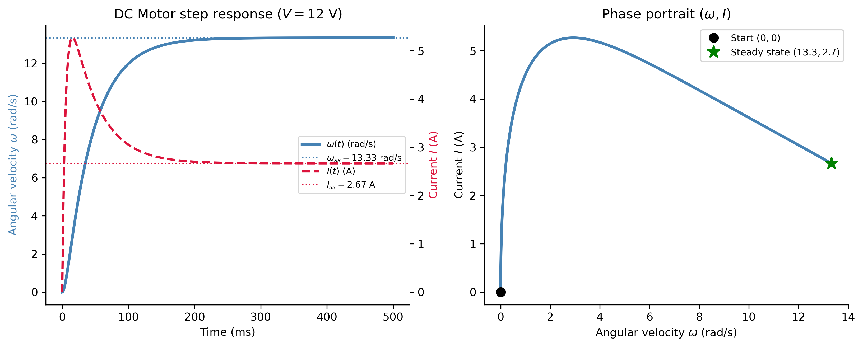
Setting all derivatives to zero in (Motor) at steady state: \[ (bR_a + K_bK_T)\,\omega_{ss} = K_T\,V_{dc} \quad\Longrightarrow\quad \omega_{ss} = \frac{K_T\,V_{dc}}{bR_a + K_bK_T}. \] Note that $K_b$ and $K_T$ are equal in SI units for an ideal motor.

Time Constants

The motor’s response is characterized by two time constants:

Electrical time constant: $\tau_e = L_a/R_a$ (how fast current builds up).
Mechanical time constant: $\tau_m = J/b$ (how fast the rotor accelerates).

In most motors $\tau_e \ll \tau_m$ (the current responds much faster than the speed), allowing a simplified first-order approximation obtained by setting $L_a \approx 0$: \[ J_{\rm eff}\,\omega' + b_{\rm eff}\,\omega = K_{\rm eff}\,V(t), \] where $J_{\rm eff} = J/(1 + K_bK_T/bR_a)$ and similar.

Show the code

# Motor parameters
La  = 0.01   # H   (armature inductance)
Ra  = 2.0    # Ω   (armature resistance)
J   = 0.01   # kg·m² (moment of inertia)
b   = 0.1    # N·m·s (viscous friction)
Kb  = 0.5    # V·s/rad (back-EMF constant)
Kt  = 0.5    # N·m/A  (torque constant)
V_dc = 12.0  # V

tau_e = La/Ra        # electrical time constant
tau_m = J/b          # mechanical time constant
print(f"tau_e = {tau_e*1e3:.1f} ms,  tau_m = {tau_m*1e3:.1f} ms")

# Steady state
omega_ss = Kt*V_dc / (b*Ra + Kb*Kt)
I_ss     = b*omega_ss / Kt
print(f"omega_ss = {omega_ss:.3f} rad/s = {omega_ss*60/(2*np.pi):.1f} RPM")
print(f"I_ss     = {I_ss:.3f} A")

def motor_ode(t, y):
    I, omega = y
    dI     = (V_dc - Ra*I - Kb*omega) / La
    domega = (Kt*I  - b*omega)        / J
    return [dI, domega]

t_plot = np.linspace(0, 0.5, 2000)
sol = solve_ivp(motor_ode, (0, 0.5), [0.0, 0.0], t_eval=t_plot, max_step=1e-4)
I_t, omega_t = sol.y

fig, axes = plt.subplots(1, 2, figsize=(11, 4.5))

# ── Time domain ──────────────────────────────────────────────
ax_tw = axes[0].twinx()
axes[0].plot(t_plot*1e3, omega_t, color='steelblue', lw=2.5, label='$\\omega(t)$ (rad/s)')
ax_tw.plot(t_plot*1e3,  I_t,     color='crimson',   lw=2, ls='--', label='$I(t)$ (A)')
axes[0].axhline(omega_ss, color='steelblue', ls=':', lw=1.2,
                label=f'$\\omega_{{ss}}={omega_ss:.2f}$ rad/s')
ax_tw.axhline(I_ss, color='crimson', ls=':', lw=1.2,
              label=f'$I_{{ss}}={I_ss:.2f}$ A')

axes[0].set_xlabel('Time (ms)')
axes[0].set_ylabel('Angular velocity $\\omega$ (rad/s)', color='steelblue')
ax_tw.set_ylabel('Current $I$ (A)', color='crimson')
axes[0].set_title('DC Motor step response ($V=12$ V)')

lines1, labels1 = axes[0].get_legend_handles_labels()
lines2, labels2 = ax_tw.get_legend_handles_labels()
axes[0].legend(lines1+lines2, labels1+labels2, fontsize=8, loc='center right')

# ── Phase portrait (omega, I) ────────────────────────────────
axes[1].plot(omega_t, I_t, color='steelblue', lw=2.5)
axes[1].plot(0, 0, 'ko', markersize=8, label='Start $(0,0)$', zorder=5)
axes[1].plot(omega_ss, I_ss, 'g*', markersize=12,
             label=f'Steady state $({omega_ss:.1f},{I_ss:.1f})$', zorder=5)
axes[1].set_xlabel('Angular velocity $\\omega$ (rad/s)')
axes[1].set_ylabel('Current $I$ (A)')
axes[1].set_title('Phase portrait $(\\omega, I)$')
axes[1].legend(fontsize=8.5)

plt.tight_layout()
plt.show()

tau_e = 5.0 ms,  tau_m = 100.0 ms
omega_ss = 13.333 rad/s = 127.3 RPM
I_ss     = 2.667 A

Figure 5: DC motor step response to $V=12$ V applied at $t=0$ (all initial conditions zero). Left: angular velocity $\omega(t)$ and armature current $I(t)$ — the current spikes immediately (electrical time constant $\tau_e=5\,\text{ms}$) while speed builds more slowly (mechanical time constant $\tau_m=100\,\text{ms}$). Right: phase portrait $(\omega, I)$ showing the trajectory from rest to steady state. Both quantities approach their analytically computed steady-state values (dashed lines).

Motor Speed Control: Varying the Input Voltage

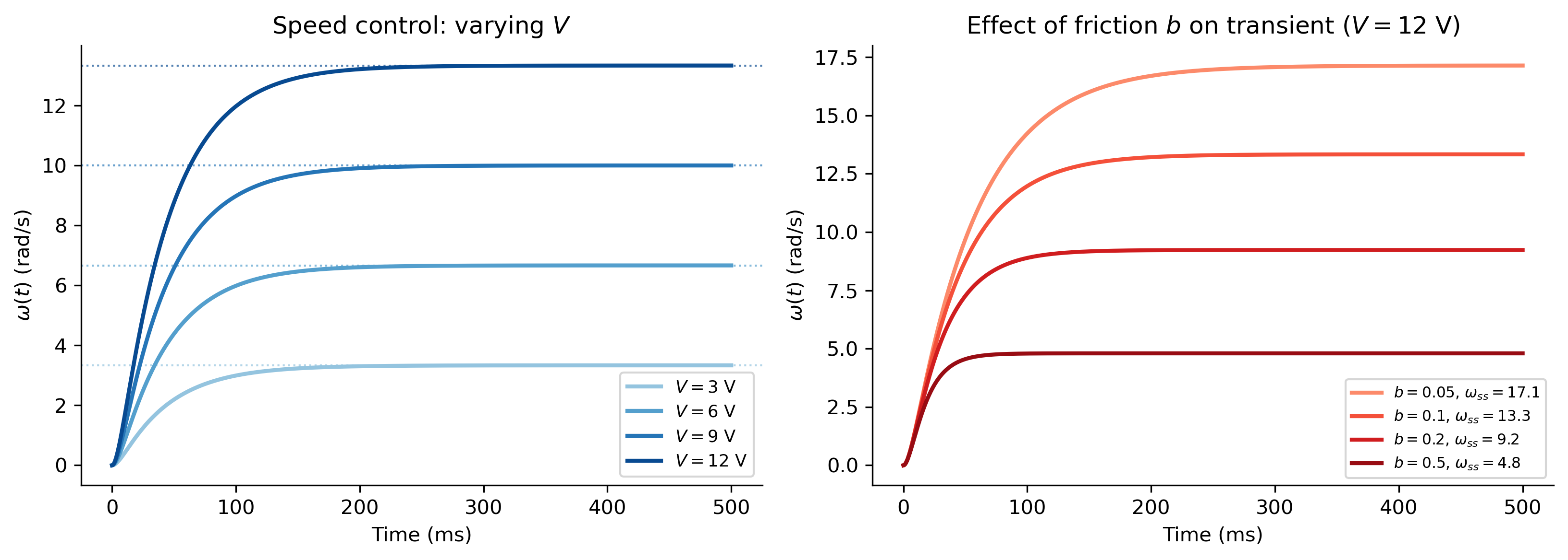
One of the most important engineering applications is speed control — choosing $V(t)$ to achieve a desired $\omega(t)$. The simplest approach uses a pulse-width modulation (PWM) signal: a square wave that switches between $0$ and $V_{dc}$ at high frequency. The average voltage $\bar{V} = D \cdot V_{dc}$ (where $D \in [0,1]$ is the duty cycle) determines the steady-state speed.

Show the code

fig, axes = plt.subplots(1, 2, figsize=(11, 4))
t_plot = np.linspace(0, 0.5, 1000)

# Varying voltage
for V_val, color, lbl in zip([3, 6, 9, 12],
                              plt.cm.Blues(np.linspace(0.4, 0.9, 4)),
                              ['$V=3$ V','$V=6$ V','$V=9$ V','$V=12$ V']):
    def motor_V(t, y, V=V_val):
        I, omega = y
        return [(V - Ra*I - Kb*omega)/La, (Kt*I - b*omega)/J]
    sol = solve_ivp(motor_V, (0,0.5), [0,0], t_eval=t_plot, max_step=1e-4)
    axes[0].plot(sol.t*1e3, sol.y[1], color=color, lw=2, label=lbl)
    omega_ss_v = Kt*V_val/(b*Ra + Kb*Kt)
    axes[0].axhline(omega_ss_v, color=color, ls=':', lw=1, alpha=0.7)

axes[0].set_xlabel('Time (ms)'); axes[0].set_ylabel('$\\omega(t)$ (rad/s)')
axes[0].set_title('Speed control: varying $V$')
axes[0].legend(fontsize=8.5)

# Varying friction
V_fixed = 12.0
for b_val, color, lbl in zip([0.05, 0.1, 0.2, 0.5],
                              plt.cm.Reds(np.linspace(0.4, 0.9, 4)),
                              ['$b=0.05$','$b=0.1$','$b=0.2$','$b=0.5$']):
    def motor_b(t, y, bv=b_val):
        I, omega = y
        return [(V_fixed - Ra*I - Kb*omega)/La, (Kt*I - bv*omega)/J]
    sol = solve_ivp(motor_b, (0,0.5), [0,0], t_eval=t_plot, max_step=1e-4)
    omega_ss_b = Kt*V_fixed/(b_val*Ra + Kb*Kt)
    axes[1].plot(sol.t*1e3, sol.y[1], color=color, lw=2,
                 label=f'{lbl}, $\\omega_{{ss}}={omega_ss_b:.1f}$')

axes[1].set_xlabel('Time (ms)'); axes[1].set_ylabel('$\\omega(t)$ (rad/s)')
axes[1].set_title('Effect of friction $b$ on transient ($V=12$ V)')
axes[1].legend(fontsize=7.5)

plt.tight_layout()
plt.show()

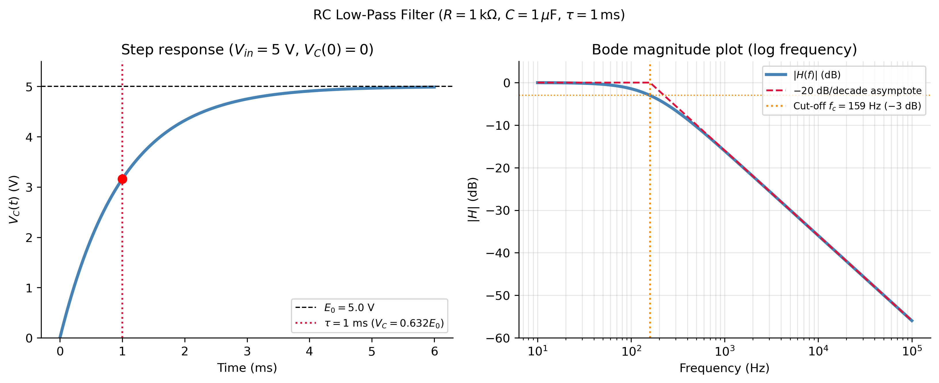
Figure 6: DC motor speed control by varying applied voltage. Left: step responses for four voltage levels — the steady-state speed scales linearly with $V$ (the motor is a linear system). Right: effect of friction coefficient $b$ on transient response with $V=12$ V — higher friction gives faster settling but lower steady-state speed.

Connecting the Three Applications

All three systems studied here are governed by linear ODEs with constant coefficients — the same equations studied in Notes 4. The following table collects the governing parameters and their roles:

	RC filter	RLC circuit	DC motor
ODE order	1st	2nd	2nd (reduced)
Natural frequency	$\omega_c=1/(RC)$	$\omega_0=1/\sqrt{LC}$	$\omega_n = \sqrt{(bR_a+K_bK_T)/(JL_a)}$
Damping	—	$\alpha = R/(2L)$	$\alpha_m = (JR_a+bL_a)/(2JL_a)$
Quality factor	—	$Q=\omega_0 L/R$	$Q_m = \omega_n/(2\alpha_m)$
Resonance	No	Yes ($Q>1/2$)	Usually overdamped
Key application	Audio/signal filtering	Radio tuning	Robotics, EVs

Looking Ahead: Systems and Laplace Transforms

The DC motor naturally leads to Chapter 3 systems of ODEs — the two coupled equations (E) and (M) form a $2\times 2$ linear system $\mathbf{y}' = A\mathbf{y} + \mathbf{b}V(t)$. The eigenvalues of the matrix $A$ determine stability and the nature of the transient (real → exponential, complex → oscillatory), exactly as for scalar second-order equations.

All three circuits here also have natural descriptions in terms of the Laplace transform — which converts the ODE into an algebraic equation in the complex frequency variable $s$, and the transfer function $H(s)$ directly encodes the frequency response. This is the starting point of classical control theory and is covered in advanced courses in signals and systems.

References

Expand for Session Info

Show the code

import sys
print("Python version:", sys.version)
print('\n'.join(f'{m.__name__}=={m.__version__}' for m in globals().values() if getattr(m, '__version__', None)))

Python version: 3.14.4 | packaged by conda-forge | (main, Apr  8 2026, 02:33:53) [Clang 20.1.8 ]
numpy==2.4.3
sympy==1.14.0
matplotlib==3.10.8

Reuse

CC BY-NC-SA 4.0

Part 1 — The RC Low-Pass Filter

Circuit Equation

Step Response

Frequency Response — The Low-Pass Filter

Part 2 — The Series RLC Circuit

Circuit Equation

The Mechanical–Electrical Correspondence

Free Response: Three Damping Regimes

Driven Response: Impedance and the Quality Factor

The Quality Factor \(Q\)

Application: The AM Radio Receiver

Part 3 — The DC Motor

Physical Setup

Governing ODEs

Reduction to a Second-Order ODE

Steady-State Speed

Time Constants

Motor Speed Control: Varying the Input Voltage

Connecting the Three Applications

References

Reuse