import numpy as npimport sympy as symimport matplotlib as mplimport matplotlib.pyplot as pltfrom scipy.integrate import solve_ivpfrom IPython.display import Math, displaympl.rcParams['figure.dpi'] =150mpl.rcParams['axes.spines.top'] =Falsempl.rcParams['axes.spines.right'] =False
When we write down a differential equation and impose an initial condition, we are implicitly making several assumptions: that a solution exists, that it is unique, and that it varies continuously with the data we prescribe. These assumptions are so natural that they are easy to take for granted — until we encounter an equation where one of them fails, and the mathematics behaves in a completely unexpected way.
This section develops the three foundational theorems for the initial value problem (IVP) for first-order ODEs. We aim for both geometric intuition and precise statements, and we trace the rich history that led to these results.
The Cauchy Problem
A first-order initial value problem (IVP), also known as the Cauchy problem in honor of its principal analyst, consists of an ODE together with a prescribed initial state: \[
\begin{cases}
x' = f(t, x), \\
x(t_0) = x_0.
\end{cases}
\tag{IVP}
\] The unknown is a function \(x = x(t)\) defined on some interval \(I\) containing \(t_0\).
What we want to know:
Existence. Does (IVP) have at least one solution?
Uniqueness. Does (IVP) have at most one solution?
Continuous dependence. If we perturb \(x_0\) slightly, does the solution change only slightly?
These three questions define what it means for a mathematical problem to be well-posed in the sense of Jacques Hadamard (1865–1963), who argued that a physically meaningful problem must have all three properties.
Historical Background
The Pre-History: Leibniz, Euler, and Bernoulli
The question of whether an ODE has a solution was not even meaningfully posed until the late 17th century, when Leibniz and Newton invented calculus. For the next century and a half, mathematicians — Leibniz, the Bernoullis, Euler, Lagrange — solved specific ODEs by constructing explicit formulas. The implicit assumption was always: if you can write down an equation, a solution must exist.
Leonhard Euler (1707–1783) took the first step toward a general theory by introducing his numerical method (now called Euler’s method) in 1768. Euler’s polygon construction approximates the solution by following the slope field in small steps. This is not just a numerical algorithm — it is a constructive proof that a solution can be approximated arbitrarily well, which was the seed of the later existence proofs.
Cauchy and the First Existence Theorem
Augustin-Louis Cauchy (1789–1857) is the towering figure in the rigorous foundation of analysis. In the 1820s he gave the first proof (using the Cauchy–Lipschitz method of successive approximations) that the IVP has a solution when \(f\) is continuous and satisfies a Lipschitz condition. His approach was formalized and extended by Rudolf Lipschitz (1832–1903), which is why the key condition bears both names.
At the same time, Cauchy introduced complex analysis as a tool for ODEs, proving existence for analytic \(f\) by power series (the Cauchy–Kovalevskaya theorem, later extended to PDEs by Sofia Kovalevskaya in 1875).
Peano and Existence Without Uniqueness
Giuseppe Peano (1858–1932), better known today for the Peano axioms of arithmetic, proved in 1886 that the IVP has at least one solution whenever \(f\) is merely continuous — no Lipschitz condition required. Peano’s theorem was a shock: continuity alone guarantees existence, but not uniqueness. His proof used a limiting argument on Euler polygon approximations.
Picard’s Fixed-Point Approach
Émile Picard (1856–1941) introduced in 1890 the method of successive approximations (now called Picard iteration): start with a constant guess \(x_0(t) = x_0\), then iterate \[
x_{n+1}(t) = x_0 + \int_{t_0}^t f\bigl(s,\, x_n(s)\bigr)\,ds.
\] When \(f\) satisfies a Lipschitz condition, this sequence converges to the unique solution — and the proof is both constructive and quantitative. Picard’s approach unified existence and uniqueness into a single elegant argument, and it is essentially the proof used today.
Gronwall and Continuous Dependence
Thomas Gronwall (1877–1932) proved his fundamental inequality in 1919, providing the technical tool needed to rigorously establish that solutions depend continuously on initial data. The Gronwall inequality has since become indispensable throughout the theory of ODEs, PDEs, and numerical analysis.
NoteTimeline
Year
Person
Contribution
1768
Euler
Euler polygon method — constructive approximation
1820s
Cauchy
First rigorous existence proof (Lipschitz condition)
1875
Kovalevskaya
Cauchy–Kovalevskaya theorem for PDEs
1876
Lipschitz
Lipschitz condition; sharpened Cauchy’s theorem
1886
Peano
Existence with continuity alone (no uniqueness)
1890
Picard
Successive approximations — unified existence + uniqueness
1919
Gronwall
Gronwall inequality — continuous dependence
The Lipschitz Condition
The hypothesis that makes the Picard–Lindelöf theorem work is the Lipschitz condition.
ImportantDefinition: Lipschitz Condition
A function \(f(t,x)\) satisfies a Lipschitz condition in \(x\) on a region \(R = \{(t,x) : |t-t_0| \leq a,\, |x-x_0| \leq b\}\) if there exists a constant \(L \geq 0\) (called the Lipschitz constant) such that \[
|f(t,x_1) - f(t,x_2)| \leq L\,|x_1 - x_2|
\] for all \((t,x_1),\, (t,x_2) \in R\).
Geometric meaning. The Lipschitz condition says the slope of \(f\) as a function of \(x\) cannot be arbitrarily steep. Think of it as a bound on how fast the vector field can tilt as you move vertically in the slope field.
Sufficient condition. If the partial derivative \(\partial f/\partial x\) exists and is bounded on \(R\), say \(|\partial f/\partial x| \leq L\), then \(f\) satisfies a Lipschitz condition with constant \(L\). This follows immediately from the Mean Value Theorem: \[
|f(t,x_1) - f(t,x_2)| = \left|\frac{\partial f}{\partial x}(t,\xi)\right| |x_1-x_2| \leq L|x_1-x_2|.
\]
NoteExamples
\(f(t,x)\)
Lipschitz in \(x\)?
Reason
\(f = ax + g(t)\)
✓
\(\partial f/\partial x = a\) bounded
\(f = t\sin(x)\)
✓ on bounded region
\(|\partial f/\partial x| = |t\cos x| \leq |t|\)
\(f = x^2\)
✓ on bounded region
\(\partial f/\partial x = 2x\) bounded if \(|x| \leq b\)
\(f = \sqrt{|x|}\)
✗ near \(x=0\)
\(\partial f/\partial x = 1/(2\sqrt{|x|}) \to \infty\)
\(f = x^{2/3}\)
✗ near \(x=0\)
derivative unbounded
The last two examples in the table are the dangerous cases — they are the ones where uniqueness can fail.
Existence and Uniqueness: The Picard–Lindelöf Theorem
Let \(f(t,x)\) be continuous on the rectangle \(R = \{(t,x): |t-t_0| \leq a,\, |x-x_0| \leq b\}\) and satisfy a Lipschitz condition in \(x\) on \(R\) with constant \(L\). Let \(M = \max_R |f(t,x)|\) and \(h = \min\!\left(a,\, b/M\right)\).
Then the IVP \(x' = f(t,x)\), \(x(t_0) = x_0\) has a unique solution \(x(t)\) on the interval \(|t - t_0| \leq h\).
Several aspects of this statement deserve comment.
Why \(h = \min(a, b/M)\)? The solution must stay inside the rectangle \(R\) where our hypotheses hold. The ODE tells us \(|x'| \leq M\), so starting from \(x_0\) the solution can travel at most \(M \cdot h\) in the \(x\)-direction in time \(h\). To stay within \(b\) of \(x_0\) we need \(Mh \leq b\), giving \(h \leq b/M\).
Local vs. global. The theorem is local — it guarantees a solution on some interval \([t_0-h, t_0+h]\), not necessarily on all of \(\mathbb{R}\). The solution can often be extended further, but may blow up in finite time (see below).
The role of continuity. Continuity of \(f\) alone (Peano’s theorem) guarantees existence but not uniqueness. The Lipschitz condition is what rules out branching.
Proof Sketch: Picard Iteration
The proof constructs the solution as the limit of the sequence: \[
x_0(t) = x_0, \qquad x_{n+1}(t) = x_0 + \int_{t_0}^t f\bigl(s,\, x_n(s)\bigr)\,ds.
\]
Step 1 — Each iterate stays in \(R\). By induction and the bound \(|x'| \leq M\), if \(x_n\) stays in \(R\) then so does \(x_{n+1}\) on \(|t-t_0| \leq h\).
Step 2 — The sequence is Cauchy. Using the Lipschitz condition repeatedly: \[
|x_{n+1}(t) - x_n(t)| \leq \frac{ML^n |t-t_0|^{n+1}}{(n+1)!} \leq \frac{ML^n h^{n+1}}{(n+1)!}.
\] The right side is the \((n+1)\)st term of the Taylor series of \(e^{Lh}\), so the series \(\sum_n |x_{n+1} - x_n|\) converges absolutely and uniformly.
Step 3 — The limit solves the IVP. Passing the limit through the integral (justified by uniform convergence), \(x(t) = \lim_{n\to\infty} x_n(t)\) satisfies the integral equation \(x(t) = x_0 + \int_{t_0}^t f(s, x(s))\,ds\), which is equivalent to the IVP.
Step 4 — Uniqueness. If two solutions \(x\) and \(\tilde{x}\) both satisfy the IVP, their difference satisfies \(|x(t) - \tilde{x}(t)| \leq L\int_{t_0}^t |x-\tilde{x}|\,ds\). The Gronwall inequality then forces \(|x(t) - \tilde{x}(t)| = 0\) for all \(t\).
The key tool in steps 2 and 4 is the Gronwall inequality, discussed below.
Picard Iteration in Practice
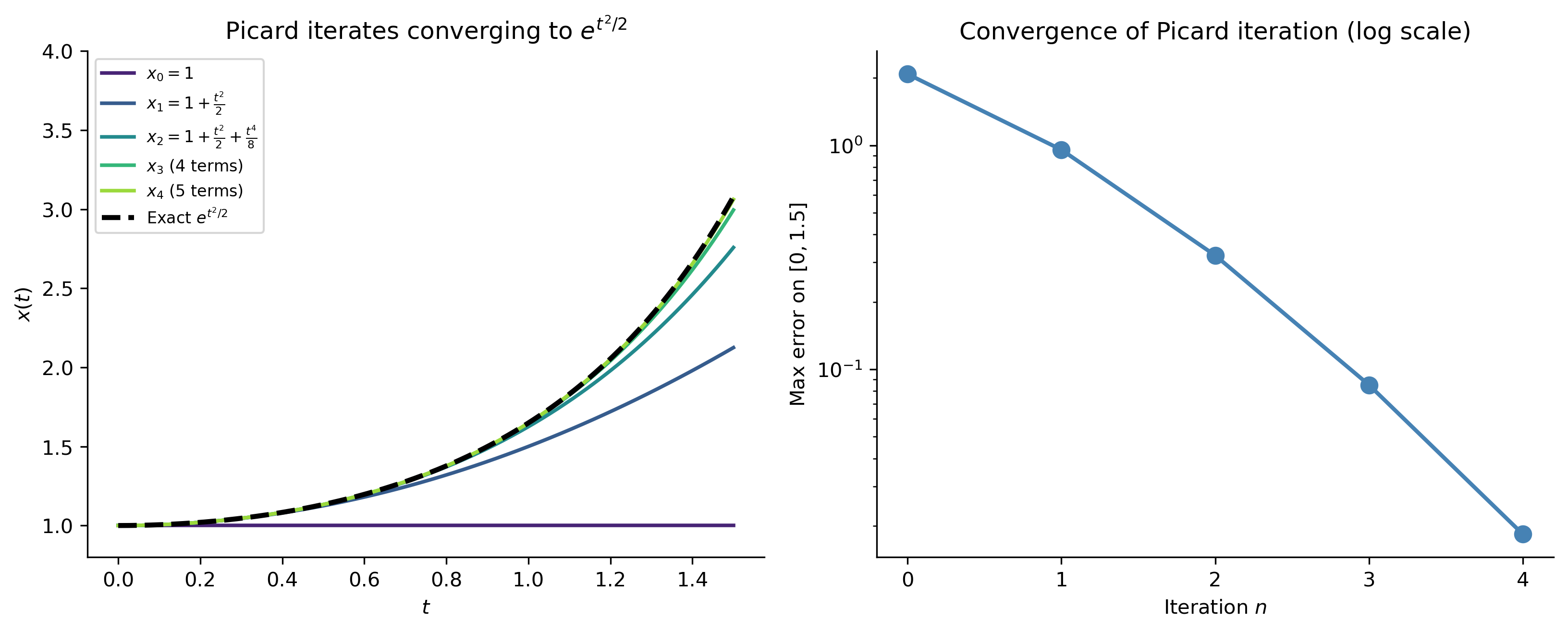
Let us watch Picard iteration converge on the simple example \(x' = tx\), \(x(0) = 1\), whose exact solution is \(x(t) = e^{t^2/2}\).
The iterates are: \[
x_0 = 1, \quad
x_1 = 1 + \frac{t^2}{2}, \quad
x_2 = 1 + \frac{t^2}{2} + \frac{t^4}{8}, \quad
x_3 = 1 + \frac{t^2}{2} + \frac{t^4}{8} + \frac{t^6}{48}, \quad \ldots
\] These are the partial sums of the Taylor series of \(e^{t^2/2}\).
Figure 1: Picard iteration for \(x'=tx\), \(x(0)=1\). Left: successive approximations \(x_0,\ldots,x_4\) (colored) converging to the exact solution \(e^{t^2/2}\) (dashed black) on \([0,1.5]\). Right: maximum error of each iterate on \([0,1.5]\) — the error decreases rapidly, confirming convergence.
When Uniqueness Fails: Peano’s Theorem and Non-Uniqueness
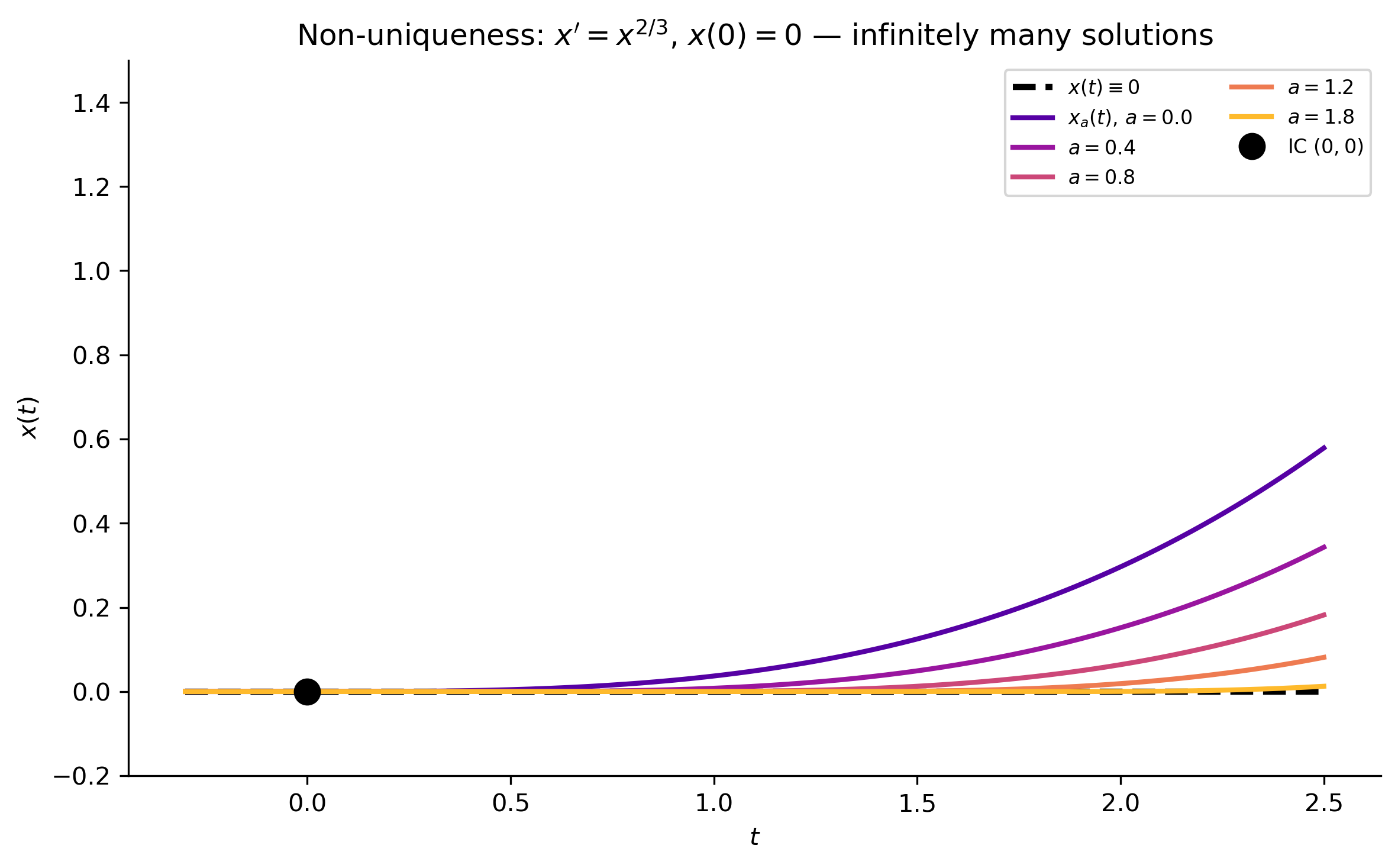
If \(f\) is continuous but not Lipschitz at \((t_0, x_0)\), then Peano’s theorem guarantees existence but uniqueness may fail. The canonical example is:
\[
x' = x^{2/3}, \qquad x(0) = 0.
\]
Here \(f(t,x) = x^{2/3}\) is continuous everywhere but \(\partial f/\partial x = \frac{2}{3}x^{-1/3}\) is unbounded near \(x = 0\) — the Lipschitz condition fails at the initial point.
Infinitely many solutions. For any \(a \geq 0\), the “glued” function \[
x_a(t) = \begin{cases} 0 & t < a \\ \left(\dfrac{t-a}{3}\right)^{\!3} & t \geq a \end{cases}
\] is continuously differentiable and satisfies the IVP. There is a one-parameter family of solutions — uniqueness fails completely.
Figure 2: Non-uniqueness for \(x' = x^{2/3}\), \(x(0)=0\). All colored curves are valid solutions of the same IVP — the Lipschitz condition fails at the origin and uniqueness is lost. Each solution stays at zero until time \(a\), then follows the cubic branch \((t-a)^3/27\).
TipGeometric Interpretation
The slope field for \(x'=x^{2/3}\) has slope \(0\) along the entire \(t\)-axis (since \(0^{2/3}=0\)), and the slope increases as \(|x|\) increases. A solution can travel along the \(t\)-axis (zero slope) indefinitely, or leave it at any time — the vector field does not “push” the solution away from \(x=0\) strongly enough to enforce a unique trajectory.
When Existence Fails: Finite-Time Blow-Up
The Picard–Lindelöf theorem guarantees a solution on some interval \([t_0-h, t_0+h]\). It does not guarantee a solution for all time. A solution may cease to exist at a finite time — it blows up.
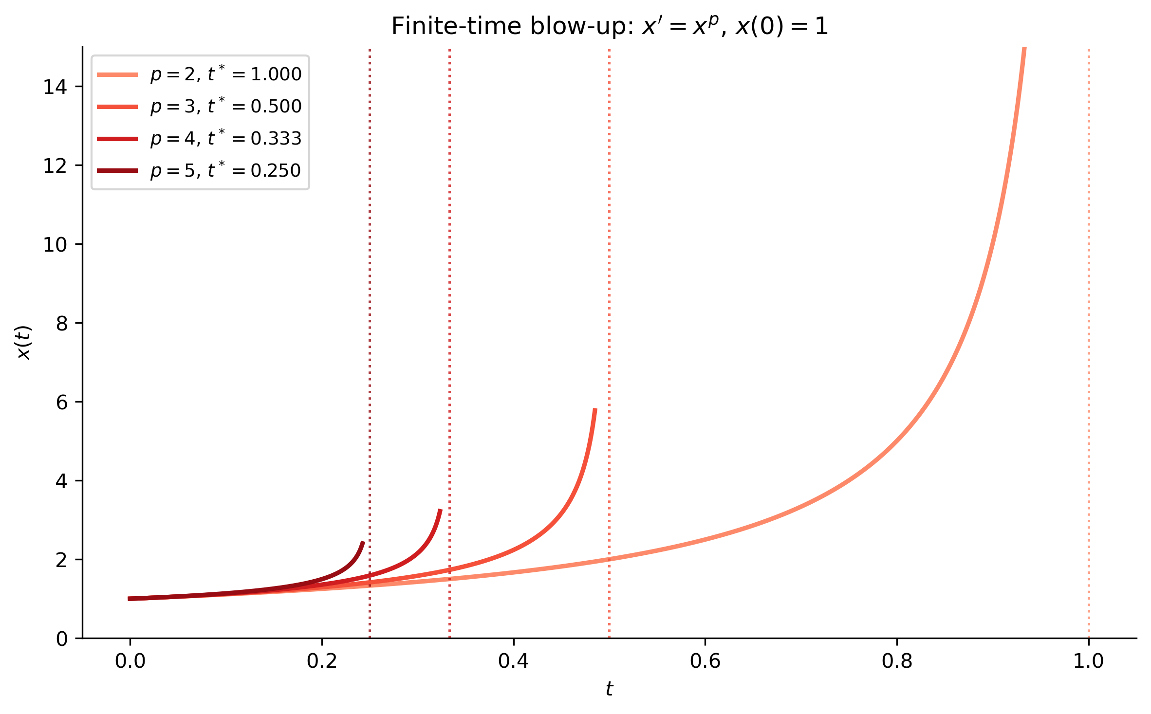
The classic example is: \[
x' = x^2, \qquad x(0) = 1 \quad\Longrightarrow\quad x(t) = \frac{1}{1-t}.
\] The solution is uniquely defined on \((-\infty, 1)\) but \(x(t) \to +\infty\) as \(t \to 1^-\). There is no way to extend the solution past \(t = 1\).
More generally, for \(x' = x^p\) with \(p > 1\) and \(x(0) = x_0 > 0\): \[
x(t) = \frac{x_0}{\bigl(1 - (p-1)x_0^{p-1}t\bigr)^{1/(p-1)}},
\qquad t < t^* = \frac{1}{(p-1)x_0^{p-1}}.
\]
Figure 3: Finite-time blow-up for \(x'=x^p\) with \(x(0)=1\). Each solution exists only up to a finite blow-up time \(t^* = 1/(p-1)\) (marked with dashed vertical lines). Solutions blow up faster for larger \(p\).
NoteMaximal Interval of Existence
The maximal interval of existence\((\alpha, \beta)\) is the largest open interval on which the solution is defined. If \(\beta < \infty\), then necessarily \(|x(t)| \to \infty\) as \(t \to \beta^-\) (the solution blows up). A solution that exists for all \(t \in \mathbb{R}\) is called a global solution.
For linear ODEs \(x' + p(t)x = q(t)\) with continuous coefficients, solutions always exist globally on any interval where \(p\) and \(q\) are continuous — blow-up is a purely nonlinear phenomenon.
Peano’s Existence Theorem
When the Lipschitz condition is dropped, we lose uniqueness but retain existence:
ImportantTheorem (Peano, 1886)
If \(f(t,x)\) is continuous on the rectangle \(R = \{|t-t_0| \leq a,\, |x-x_0| \leq b\}\), then the IVP \(x' = f(t,x)\), \(x(t_0) = x_0\) has at least one solution on \(|t-t_0| \leq h\), where \(h = \min(a, b/M)\) and \(M = \max_R |f|\).
Proof idea. Construct Euler polygon approximations \(x^{(n)}\) with step size \(1/n\). Each \(x^{(n)}\) is continuous, uniformly bounded, and equicontinuous (slopes bounded by \(M\)). The Arzelà–Ascoli theorem guarantees a uniformly convergent subsequence, and the limit is a solution.
Peano’s theorem shows that continuity is the minimal condition for existence. The gap between Peano and Picard–Lindelöf — the Lipschitz condition — is precisely what separates existence from uniqueness.
Continuous Dependence on Initial Conditions
The third pillar of well-posedness asks: if we perturb \(x_0\) by a small amount \(\delta\), does the solution change by at most a small amount (depending continuously on \(\delta\))?
ImportantTheorem (Continuous Dependence)
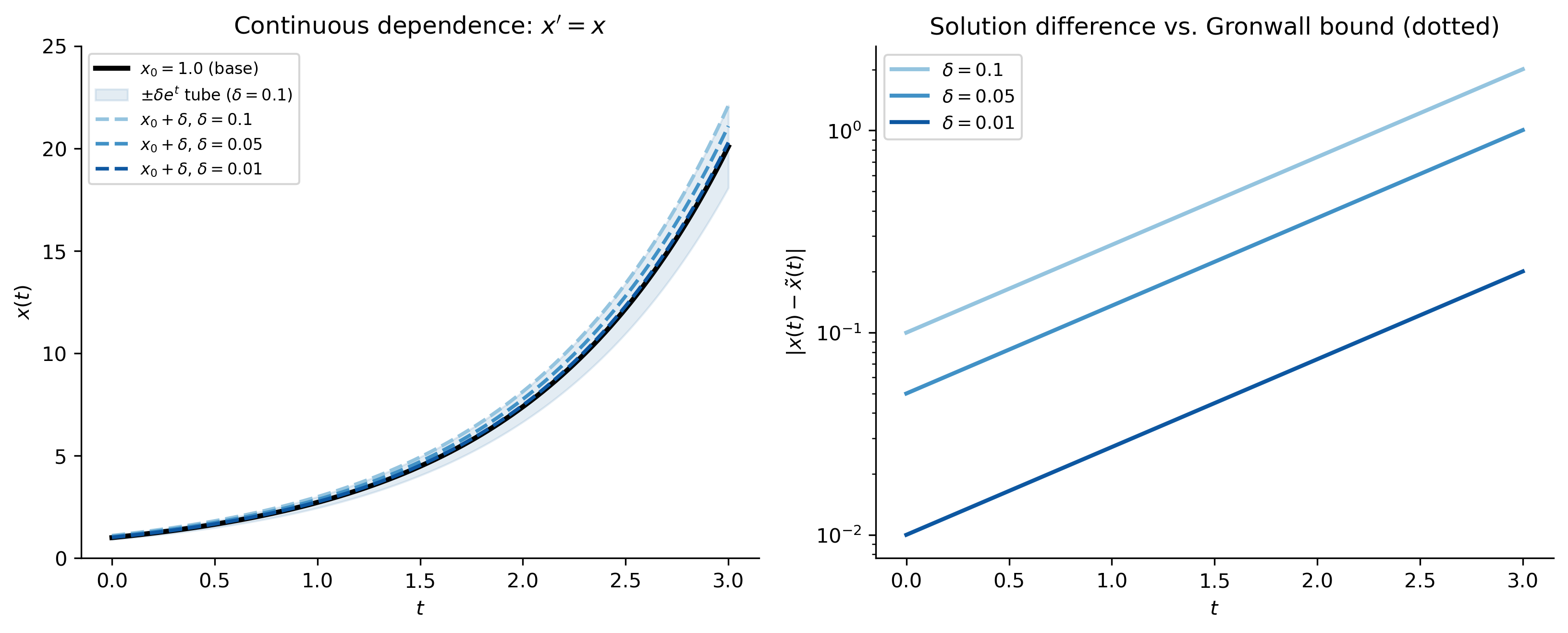
Under the hypotheses of the Picard–Lindelöf theorem, let \(x(t)\) be the solution to the IVP with initial condition \(x(t_0) = x_0\), and let \(\tilde{x}(t)\) be the solution with \(\tilde{x}(t_0) = \tilde{x}_0\). Then for \(|t - t_0| \leq h\): \[
|x(t) - \tilde{x}(t)| \leq |\tilde{x}_0 - x_0|\,e^{L|t-t_0|}.
\] In particular, if \(|\tilde{x}_0 - x_0| < \delta\), then \(|x(t) - \tilde{x}(t)| < \delta\,e^{Lh}\) — a bound proportional to \(\delta\).
The exponential factor \(e^{L|t-t_0|}\) says that solutions can diverge — small initial differences can grow — but they grow at most exponentially, and on a bounded time interval the bound is finite.
The Gronwall Inequality
The key technical tool for continuous dependence (and for the uniqueness part of Picard–Lindelöf) is the following remarkable inequality.
ImportantGronwall’s Inequality (1919)
Let \(u(t) \geq 0\) be continuous on \([t_0, T]\), and suppose \[
u(t) \leq \alpha + \beta \int_{t_0}^t u(s)\,ds
\] for constants \(\alpha \geq 0\), \(\beta \geq 0\). Then \[
u(t) \leq \alpha\,e^{\beta(t-t_0)} \quad \text{for all } t \in [t_0, T].
\]
How it proves continuous dependence. Let \(u(t) = |x(t) - \tilde{x}(t)|\). Subtracting the integral equations for \(x\) and \(\tilde{x}\) and using the Lipschitz condition: \[
u(t) \leq |\tilde{x}_0 - x_0| + L\int_{t_0}^t u(s)\,ds.
\] This is exactly Gronwall’s inequality with \(\alpha = |\tilde{x}_0 - x_0|\) and \(\beta = L\), giving \(u(t) \leq |\tilde{x}_0 - x_0|\,e^{L(t-t_0)}\).
Figure 4: Continuous dependence for \(x'=x\), \(x(0)=x_0\). Left: solutions from three nearby initial conditions — small initial separation grows but remains controlled on any bounded interval. Right: the difference between each perturbed solution and the base solution \(x_0=1\) matches the Gronwall bound \(\delta e^t\) exactly (as expected since \(L=1\) for this linear ODE).
Sensitivity to Initial Conditions and Chaos
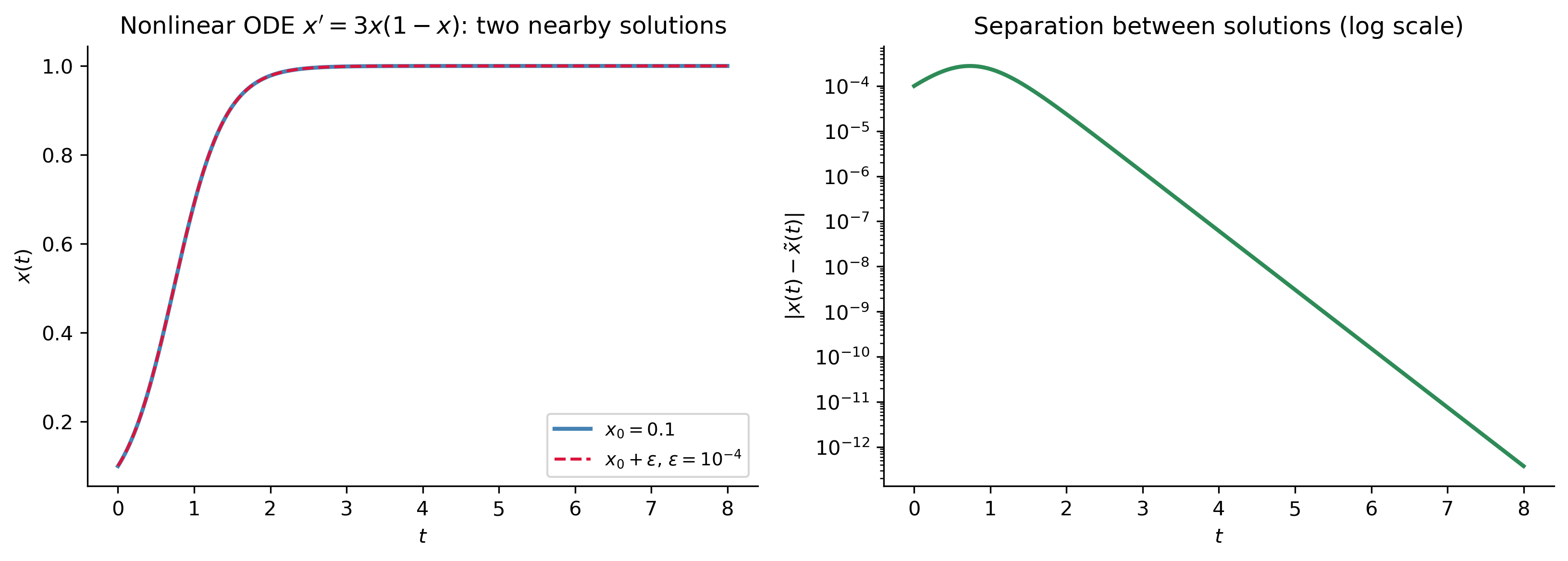
The exponential factor \(e^{L(t-t_0)}\) in the continuous dependence bound is sharp: even for the simple linear equation \(x' = x\), the separation between two solutions starting \(\delta\) apart grows as \(\delta e^t\). On long time intervals this can be enormous.
For nonlinear systems, the effective Lipschitz constant can be large, or can vary in time, leading to sensitive dependence on initial conditions — the hallmark of chaos. In a chaotic system, two trajectories starting arbitrarily close diverge exponentially fast, making long-term prediction practically impossible.
The quantitative measure of this divergence is the Lyapunov exponent\(\lambda\): on average, nearby trajectories separate as \(e^{\lambda t}\). A positive Lyapunov exponent signals chaos. Famous chaotic systems include the Lorenz equations (a simplified model of atmospheric convection) and the double pendulum.
Note
The existence and uniqueness theorem still holds for chaotic systems — the IVP has a unique solution. Chaos is not about non-uniqueness; it is about the sensitivity of that unique solution to the initial condition. Uniqueness and chaos are perfectly compatible.
Figure 5: Sensitive dependence: logistic ODE \(x'=3x(1-x)\) from two initial conditions differing by \(\varepsilon = 10^{-4}\). On a short interval both solutions track each other closely; on a longer interval they diverge noticeably, illustrating how even well-posed, unique solutions can be sensitive to tiny perturbations in a nonlinear setting.
Why These Theorems Matter
In Mathematics
The existence and uniqueness theorems are the bedrock of the entire theory of ODEs.
They justify the general solution concept: a 1st-order ODE has a one-parameter family of solutions because a unique solution is determined by one piece of initial data. Without uniqueness, the notion of a “general solution” containing all solutions would be meaningless.
They underpin qualitative theory: phase plane analysis, stability theory, and bifurcation theory all assume solutions are unique, so trajectories cannot cross in the phase plane.
They drive numerical methods: Euler’s method, Runge–Kutta, and all modern ODE solvers are justified by the fact that they approximate a unique, continuously dependent solution. Error bounds for numerical methods are derived using the Gronwall inequality.
They extend to higher-order ODEs and systems: a 2nd-order ODE requires two initial conditions for a unique solution; an \(n\times n\) system requires \(n\) initial conditions. The same Picard–Lindelöf framework applies.
In Physics and Engineering
TipDeterminism
In classical mechanics, Newton’s second law \(m\ddot{\mathbf{r}} = \mathbf{F}(\mathbf{r}, \dot{\mathbf{r}}, t)\) is a system of ODEs. Uniqueness is the mathematical statement of determinism: knowing the position and velocity of every particle at one instant completely determines all past and future motion. This was the philosophical foundation of the Laplacian worldview — the universe as a clockwork whose future is in principle fully predictable.
Control systems. A controller can only stabilize a system if the system responds predictably to inputs. Continuous dependence on initial conditions guarantees this predictability on finite time intervals.
Simulation and modeling. Every numerical simulation of a physical system — weather forecasting, circuit simulation, structural analysis, fluid dynamics — rests on the assumption that the governing equations are well-posed. If existence or uniqueness failed, no numerical method could converge to a meaningful answer.
Sensitivity analysis and uncertainty quantification. The Gronwall bound provides explicit estimates for how initial measurement errors propagate through a simulation. These estimates are used in engineering to determine required measurement precision.
The limits of predictability. For chaotic systems the Gronwall bound is exponentially growing, which means initial measurement errors amplify exponentially. This is why weather forecasts are reliable for a few days but not for months — not because solutions fail to exist or be unique, but because the exponential sensitivity makes the unique solution practically unpredictable from imprecise data.
Summary
Theorem
Hypothesis
Conclusion
Peano (1886)
\(f\) continuous
At least one solution exists locally
Picard–Lindelöf
\(f\) continuous + Lipschitz in \(x\)
Unique solution exists locally
Continuous dependence
\(f\) continuous + Lipschitz in \(x\)
Solutions vary continuously with \(x_0\); bound \(\delta e^{L(t-t_0)}\)
Global existence
\(f\) linear in \(x\)
Solutions exist on entire interval of continuity of \(p(t)\), \(q(t)\)
ImportantKey Takeaways
Continuity of \(f\) is sufficient for existence (Peano), but not for uniqueness.
Lipschitz continuity of \(f\) in \(x\) — equivalently, boundedness of \(\partial f/\partial x\) — is the additional condition that gives uniqueness.
Uniqueness fails when \(\partial f/\partial x\) is unbounded near the initial point (e.g., \(f = x^{2/3}\) at \(x=0\)).
Existence fails globally for nonlinear equations: solutions can blow up in finite time. This never happens for linear equations.
Continuous dependence is guaranteed on any bounded interval, with an explicit exponential bound derived from the Gronwall inequality.
Chaos is consistent with well-posedness: unique solutions can still be exponentially sensitive to initial conditions.
Relevant Videos
Existence and uniqueness:
References
TipExpand for Session Info
Show the code
import sysprint("Python version:", sys.version)print('\n'.join(f'{m.__name__}=={m.__version__}'for m inglobals().values() ifgetattr(m, '__version__', None)))