Draining Tanks, Coupled Reservoirs, and Drag

Fluid-Dynamics Applications of ODEs

Show the code
import numpy as np
import sympy as sym
import matplotlib as mpl
import matplotlib.pyplot as plt
from scipy.integrate import solve_ivp
from scipy.optimize import fsolve
from IPython.display import Math, display
mpl.rcParams['figure.dpi'] = 150
mpl.rcParams['axes.spines.top'] = False
mpl.rcParams['axes.spines.right'] = False

Fluid mechanics at the center of engineering applications (fluid mechanics, thermo-fluids, hydraulics, HVAC, and process control for MEs; sensors, actuators, and process instrumentation for EEs). It turns out that fluid systems reuse essentially every ODE technique in this course — first-order separable equations, first-order linear systems, nonlinear systems, numerical methods, and (in the optional capstone) Laplace transforms. This section develops four core applications, plus one optional capstone, each keyed to a specific part of the syllabus.

  1. Torricelli’s Law — a tank draining through a hole is a first-order nonlinear separable ODE (Notes 2), and it behaves qualitatively differently from the linear decay models you have already seen.
  2. Coupled tanks with laminar valves — two interconnected reservoirs form a first-order linear system (Chapter 3), and the flow is governed by the exact same mathematics as an RC/RLC network — the hydraulic–electrical analogy made explicit.
  3. Coupled tanks with turbulent valves — the same two tanks, but with a nonlinear (square-root) interconnection, giving a genuine nonlinear system: equilibria, linearization/stability, and a hands-on comparison of Euler’s method against RK4 (Numerical Methods).
  4. Motion through a fluid — a falling object experiences either linear (Stokes) or quadratic (form) drag depending on the Reynolds number, giving a clean side-by-side example of a linear vs. a nonlinear first-order model of the same physical process.
  5. (Optional capstone) The surge tank — a linear second-order ODE describing pressure-relief oscillations in a hydropower penstock, solved with the Laplace transform.

Part 1 — Torricelli’s Law: Draining a Tank

Physical Setup

Consider a tank with constant cross-sectional area \(A\), filled with liquid to height \(h(t)\), draining through a small hole of area \(a\) in the bottom. Torricelli’s law (derivable from Bernoulli’s equation applied between the free surface and the orifice) states that liquid exits the hole with speed \[ v = \sqrt{2gh}. \] The volumetric outflow rate is \(Q = C_d\,a\,v\), where \(C_d\) is a discharge coefficient (\(C_d \approx 0.6\text{–}0.8\) for a sharp-edged orifice) that accounts for the contraction of the exiting jet and other real-world losses. Conservation of volume (\(A\,dh = -Q\,dt\)) gives \[ A\,\frac{dh}{dt} = -C_d\,a\sqrt{2g}\,\sqrt{h}. \] Lumping the constants into \(k = C_d\,a\sqrt{2g}/A\): \[ \boxed{\frac{dh}{dt} = -k\sqrt{h}.} \tag{Torricelli} \]

Solving the ODE

This equation is first-order and separable, but — unlike every “decay” model you have seen so far (radioactive decay, Newton’s law of cooling, RC circuits) — it is nonlinear, because \(\sqrt{h}\) is not proportional to \(h\). Separating variables, \[ \int h^{-1/2}\,dh = -k\int dt \quad\Longrightarrow\quad 2\sqrt{h} = -kt + 2\sqrt{h_0}, \] so \[ \boxed{h(t) = \left(\sqrt{h_0} - \frac{k}{2}t\right)^{\!2}, \qquad 0 \le t \le T,} \] where \(h_0 = h(0)\) and \[ T = \frac{2\sqrt{h_0}}{k} \] is the drain time — the tank empties in finite time.

NoteA New Kind of Long-Term Behavior

Every linear first-order model in Notes 2 (exponential growth/decay, RC charging) approaches its equilibrium asymptotically — it gets arbitrarily close but never technically arrives at \(t=\infty\). Torricelli’s equation is qualitatively different: because the right-hand side is only Hölder continuous (not Lipschitz) at \(h=0\), the solution reaches \(h=0\) in finite time and stays there (\(dh/dt=0\) once \(h=0\), so the tank does not “go negative”). If you plug \(t>T\) into the boxed formula above, the algebra produces \(h(t) = \left(\tfrac{k}{2}t - \sqrt{h_0}\right)^2 > 0\) again — a tank mysteriously refilling itself! This is not a contradiction; it simply means the formula is only a valid solution to the physical problem on \(0 \le t \le T\). Past \(T\), the correct physical solution is \(h(t)\equiv 0\). Always check the domain of validity of a solution against the physics of the problem, not just against the algebra.

Show the code
g   = 9.81
A_t = 0.20      # m^2  (tank cross-section, ~50 cm diameter)
a_t = 1.0e-4    # m^2  (orifice, ~1.1 cm diameter hole)
Cd  = 0.6
h0  = 1.0       # m

k_t = Cd*a_t*np.sqrt(2*g)/A_t
T_t = 2*np.sqrt(h0)/k_t
print(f"k = {k_t:.6f} m^0.5/s,  drain time T = {T_t:.1f} s = {T_t/60:.2f} min")

def h_analytic(t):
    return np.maximum(np.sqrt(h0) - k_t*t/2, 0.0)**2

def tank_ode(t, h):
    return [-k_t*np.sqrt(max(h[0], 0.0))]

t_num = np.linspace(0, T_t, 400)
sol = solve_ivp(tank_ode, (0, T_t), [h0], t_eval=t_num, max_step=1.0)

fig, axes = plt.subplots(1, 2, figsize=(11, 4.5))

# ── Physical solution vs. numerical check ───────────────────────
t_plot = np.linspace(0, T_t, 400)
axes[0].plot(t_plot/60, h_analytic(t_plot), color='steelblue', lw=2.5, label='Analytic $h(t)$')
axes[0].plot(sol.t[::20]/60, sol.y[0][::20], 'o', color='darkorange',
             ms=5, label='Numerical (solve\\_ivp)', zorder=5)
axes[0].axvline(T_t/60, color='crimson', ls=':', lw=1.5, label=f'$T={T_t/60:.1f}$ min')
axes[0].set_xlabel('Time (min)'); axes[0].set_ylabel('$h(t)$ (m)')
axes[0].set_title('Physical solution: tank empties at $t=T$')
axes[0].legend(fontsize=8.5); axes[0].set_ylim(-0.05, 1.05)

# ── Domain-of-validity issue ─────────────────────────────────
t_ext = np.linspace(0, 1.6*T_t, 400)
h_naive = (np.sqrt(h0) - k_t*t_ext/2)**2       # never clipped at 0
axes[1].plot(t_ext/60, h_naive, color='gray', ls='--', lw=2, label='Naive formula (unclipped)')
axes[1].plot(t_plot/60, h_analytic(t_plot), color='steelblue', lw=2.5, label='Physical solution')
axes[1].axvline(T_t/60, color='crimson', ls=':', lw=1.5, label=f'$T={T_t/60:.1f}$ min')
axes[1].set_xlabel('Time (min)'); axes[1].set_ylabel('$h(t)$ (m)')
axes[1].set_title('Formula continued past $T$: unphysical rebound')
axes[1].legend(fontsize=8.5)

plt.tight_layout()
plt.show()
k = 0.001329 m^0.5/s,  drain time T = 1505.1 s = 25.08 min
Figure 1: Draining a cylindrical tank (\(A=0.20\,\text{m}^2\), orifice \(a=1\,\text{cm}^2\), \(C_d=0.6\), \(h_0=1\) m). Left: the physical solution \(h(t)\) (solid) reaches zero at the drain time \(T\approx 25.1\) min and stays there, matching a direct numerical integration of the ODE (markers). Right: naively evaluating the closed-form parabola past \(t=T\) (dashed) produces an unphysical rebound — a reminder to always check a solution’s domain of validity.

Extension: Non-Cylindrical Tanks

If the tank’s cross-sectional area depends on height, \(A=A(h)\), the same volume-conservation argument gives the more general separable equation \[ A(h)\,\frac{dh}{dt} = -C_d\,a\sqrt{2g}\,\sqrt{h} = -k_0\sqrt{h}, \qquad k_0 = C_d\,a\sqrt{2g}. \]

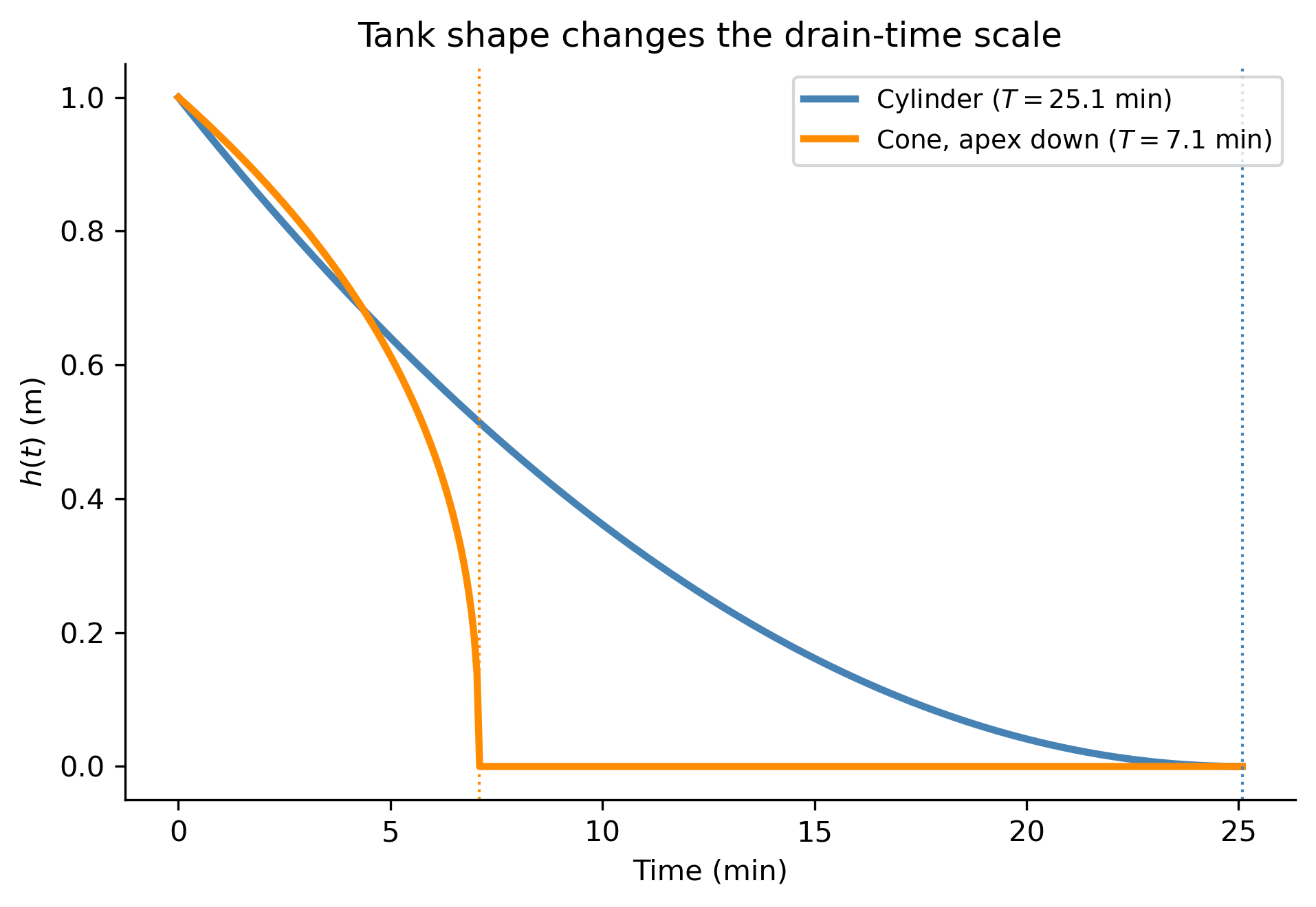
For example, an inverted cone of top radius \(R\) and height \(H\) (apex at the bottom, where the drain is located) has \(A(h) = \pi (R/H)^2 h^2\), so \[ \pi\left(\frac{R}{H}\right)^{\!2} h^{3/2}\,dh = -k_0\,dt. \] Integrating with \(h(0)=H\), \[ \boxed{h(t) = \left[H^{5/2} - \frac{5k_0}{2\pi(R/H)^2}\,t\right]^{2/5}, \qquad 0\le t\le T_{\text{cone}},} \] with drain time \(T_{\text{cone}} = \dfrac{2\pi (R/H)^2 H^{5/2}}{5k_0}\). The same separation-of-variables technique applies to any tank shape; only the integral on the left changes.

Show the code
R_cone = 0.3
H_cone = 1.0
k0 = Cd*a_t*np.sqrt(2*g)

def h_cone(t):
    coef = np.pi*(R_cone/H_cone)**2*(2/5)
    val = np.maximum(H_cone**2.5 - (k0/coef)*t, 0.0)
    return val**(2/5)

T_cone = np.pi*(R_cone/H_cone)**2*(2/5)*H_cone**2.5/k0
print(f"Cylinder drain time: {T_t/60:.2f} min   |   Cone drain time: {T_cone/60:.2f} min")

t_plot2 = np.linspace(0, T_t, 400)
fig, ax = plt.subplots(figsize=(6.5, 4.5))
ax.plot(t_plot2/60, h_analytic(t_plot2), color='steelblue', lw=2.5,
        label=f'Cylinder ($T={T_t/60:.1f}$ min)')
ax.plot(t_plot2/60, h_cone(t_plot2), color='darkorange', lw=2.5,
        label=f'Cone, apex down ($T={T_cone/60:.1f}$ min)')
ax.axvline(T_cone/60, color='darkorange', ls=':', lw=1)
ax.axvline(T_t/60, color='steelblue', ls=':', lw=1)
ax.set_xlabel('Time (min)'); ax.set_ylabel('$h(t)$ (m)')
ax.set_title('Tank shape changes the drain-time scale')
ax.legend(fontsize=9)
plt.tight_layout()
plt.show()
Cylinder drain time: 25.08 min   |   Cone drain time: 7.09 min
Figure 2: Same orifice and initial height, two tank shapes. The cone (apex-down, top radius \(R=0.3\) m at \(H=1\) m) holds only a third of the cylinder’s volume at \(h=1\) m, so it drains in about 7.1 min versus 25.1 min for the cylinder — the same \(k_0\), but a very different \(A(h)\), changes the whole time scale.

Part 2 — Coupled Tanks: Linear Systems and the Hydraulic–Electrical Analogy

Physical Setup

Now connect two tanks in series: tank 1 is fed by a constant inflow \(q_{in}\) and drains into tank 2 through a valve; tank 2 drains to atmosphere through a second valve. If both valves are laminar (a good approximation for narrow tubes, capillaries, or partially-closed valves at low flow), the flow through a valve is proportional to the pressure-head difference across it — the fluid analog of Ohm’s law: \[ Q = \frac{\Delta h}{R}, \] where \(R\) is a hydraulic resistance. With \(A_1, A_2\) the tank cross-sections and \(R_{12}, R_2\) the two valve resistances, \[ \boxed{ A_1\frac{dh_1}{dt} = q_{in} - \frac{h_1-h_2}{R_{12}}, \qquad A_2\frac{dh_2}{dt} = \frac{h_1-h_2}{R_{12}} - \frac{h_2}{R_2}. } \tag{Tanks–Linear} \] This is a first-order linear system \(\mathbf{h}' = A\mathbf{h} + \mathbf{b}\) — exactly the Chapter 3 material — with \[ A = \begin{pmatrix} -\dfrac{1}{A_1 R_{12}} & \dfrac{1}{A_1 R_{12}} \\[2mm] \dfrac{1}{A_2 R_{12}} & -\dfrac{1}{A_2 R_{12}} - \dfrac{1}{A_2 R_2} \end{pmatrix}, \qquad \mathbf{b} = \begin{pmatrix} q_{in}/A_1 \\ 0 \end{pmatrix}. \]

The Hydraulic–Electrical Analogy

Compare (Tanks–Linear) to the RC circuit equation from Topics 6: \(RC\,V_C' + V_C = V_{in}(t)\). The correspondence is exact — a fluid reservoir with a resistive drain is literally the same differential equation as a capacitor discharging through a resistor:

Fluid system Electrical system
Height \(h\) Voltage \(V\)
Flow rate \(Q\) Current \(I\)
Tank area \(A\) Capacitance \(C\)
Valve resistance \(R\) Resistance \(R\)

A tank stores fluid volume the way a capacitor stores charge; a laminar valve dissipates head the way a resistor dissipates voltage. Any student comfortable with RC circuits (Topics 6, Part 1) already understands the qualitative behavior of a single draining/filling tank with a linear valve, and — as we will see below — the coupled-tank system behaves like a two-capacitor RC network, not like an RLC circuit, because nothing in a tank-and-valve system stores fluid momentum the way an inductor stores magnetic energy. There is no hydraulic analog of \(L\) here, which is exactly why (as shown below) this system cannot oscillate.

Equilibrium and Eigenvalues

Setting \(\mathbf{h}'=\mathbf{0}\) gives the steady-state heights \(h_{1,eq} = q_{in}(R_{12}+R_2)\), \(h_{2,eq} = q_{in}R_2\) — both tanks settle to a constant fill level determined entirely by the inflow rate and the two resistances. The transient behavior is governed by the eigenvalues of \(A\):

Show the code
A1 = A2 = 1.0     # m^2
R12 = 5.0         # s/m^2
R2  = 10.0        # s/m^2
qin = 0.1         # m^3/s

Amat = np.array([[-1/(A1*R12), 1/(A1*R12)],
                  [1/(A2*R12), -1/(A2*R12) - 1/(A2*R2)]])
bvec = np.array([qin/A1, 0.0])

eigval, eigvec = np.linalg.eig(Amat)
h_eq = np.linalg.solve(-Amat, bvec)

print("A =\n", Amat)
print("eigenvalues:", eigval)
print("equilibrium (h1_eq, h2_eq):", h_eq)
A =
 [[-0.2  0.2]
 [ 0.2 -0.3]]
eigenvalues: [-0.04384472 -0.45615528]
equilibrium (h1_eq, h2_eq): [1.5 1. ]

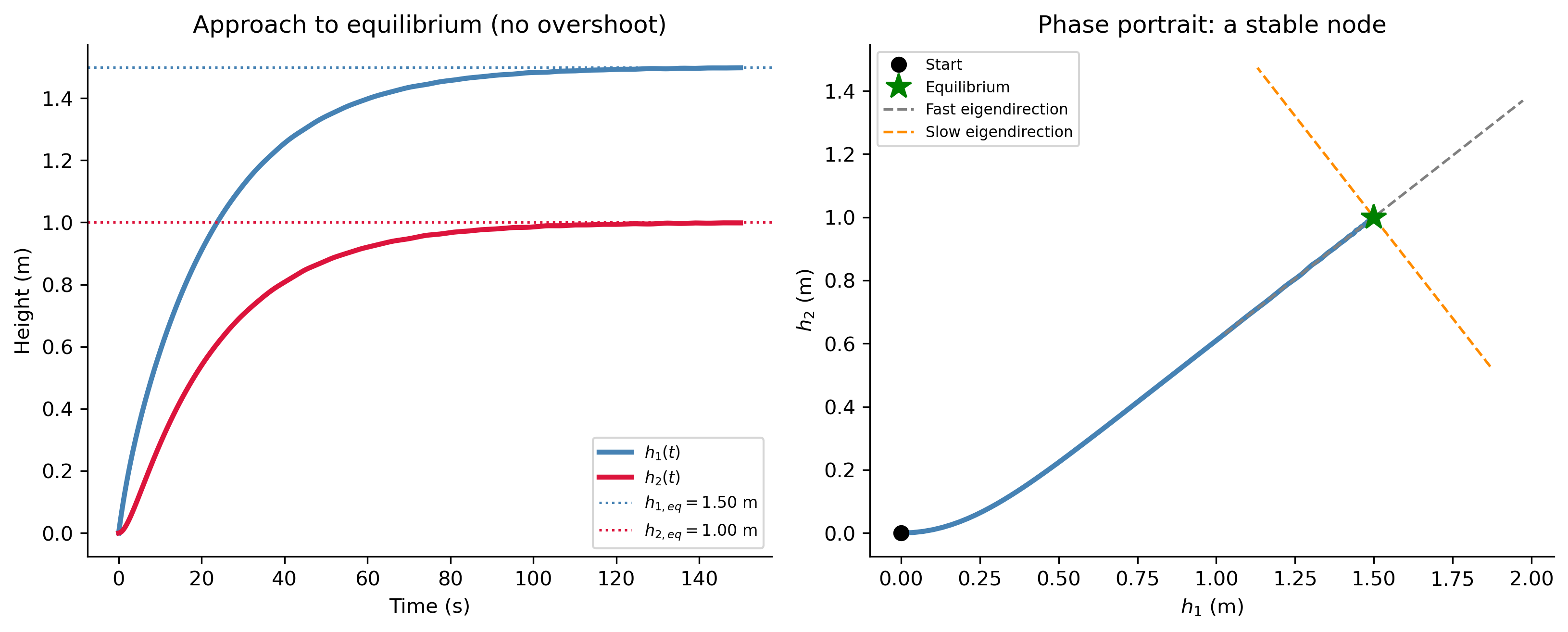
Both eigenvalues are real and negative (\(\lambda_1\approx-0.044\), \(\lambda_2\approx-0.456\) for the parameters above) — this is a stable node, exactly as you would expect for two resistively-coupled first-order storage elements. The system approaches equilibrium monotonically; unlike the RLC circuit, it can never overshoot or oscillate, because doing so would require an inertial (second-derivative) term that this model simply does not have.

Show the code
def linear_tanks(t, h):
    return Amat @ h + bvec

t_span = (0, 150)
t_eval = np.linspace(*t_span, 400)
sol_lin = solve_ivp(linear_tanks, t_span, [0.0, 0.0], t_eval=t_eval)

fig, axes = plt.subplots(1, 2, figsize=(11, 4.5))

axes[0].plot(sol_lin.t, sol_lin.y[0], color='steelblue', lw=2.5, label='$h_1(t)$')
axes[0].plot(sol_lin.t, sol_lin.y[1], color='crimson', lw=2.5, label='$h_2(t)$')
axes[0].axhline(h_eq[0], color='steelblue', ls=':', lw=1.2, label=f'$h_{{1,eq}}={h_eq[0]:.2f}$ m')
axes[0].axhline(h_eq[1], color='crimson', ls=':', lw=1.2, label=f'$h_{{2,eq}}={h_eq[1]:.2f}$ m')
axes[0].set_xlabel('Time (s)'); axes[0].set_ylabel('Height (m)')
axes[0].set_title('Approach to equilibrium (no overshoot)')
axes[0].legend(fontsize=8)

axes[1].plot(sol_lin.y[0], sol_lin.y[1], color='steelblue', lw=2.5)
axes[1].plot(0, 0, 'ko', ms=7, label='Start', zorder=5)
axes[1].plot(h_eq[0], h_eq[1], 'g*', ms=13, label='Equilibrium', zorder=5)
# eigenvector directions through the equilibrium
for lam, vec, color, lbl in zip(eigval, eigvec.T, ['gray', 'darkorange'],
                                 ['Fast eigendirection', 'Slow eigendirection']):
    pts = np.array([h_eq - 0.6*vec, h_eq + 0.6*vec])
    axes[1].plot(pts[:,0], pts[:,1], color=color, ls='--', lw=1.3, label=lbl)
axes[1].set_xlabel('$h_1$ (m)'); axes[1].set_ylabel('$h_2$ (m)')
axes[1].set_title('Phase portrait: a stable node')
axes[1].legend(fontsize=7.5)

plt.tight_layout()
plt.show()
Figure 3: Two laminar-valve tanks starting empty (\(A_1=A_2=1\,\text{m}^2\), \(R_{12}=5\), \(R_2=10\), \(q_{in}=0.1\,\text{m}^3/\text{s}\)). Left: \(h_1(t)\) and \(h_2(t)\) rise monotonically to their equilibrium values (dashed) — no overshoot is possible. Right: phase portrait \((h_1,h_2)\); the trajectory approaches equilibrium along the slow eigendirection (\(\lambda_2\approx-0.044\)), the signature of a stable node.
TipLooking Ahead: Systems Theory

This is a direct, physically transparent illustration of everything Chapter 3 teaches about linear systems: eigenvalues determine stability and the type of equilibrium (here, a stable node because both eigenvalues are real and negative); eigenvectors determine the geometry of the approach (the “slow” and “fast” directions visible in the phase portrait); and the particular/steady-state solution is found by solving the algebraic system \(A\mathbf{h}_{eq}+\mathbf{b}=\mathbf{0}\).


Part 3 — Nonlinear Coupled Tanks: A Bridge to Numerical Methods

Turbulent Valves

The linear (laminar) valve law \(Q=\Delta h/R\) only holds at low flow speeds. Most real valves and orifices operate in the turbulent regime, where — just as in Part 1 — flow is proportional to \(\sqrt{|\Delta h|}\) rather than to \(\Delta h\) itself: \[ Q = c\,\operatorname{sgn}(\Delta h)\sqrt{|\Delta h|}. \] Replacing both valves in the two-tank system with turbulent valves gives \[ \boxed{ A_1\frac{dh_1}{dt} = q_{in} - c_{12}\sqrt{h_1-h_2}, \qquad A_2\frac{dh_2}{dt} = c_{12}\sqrt{h_1-h_2} - c_2\sqrt{h_2} } \tag{Tanks–Nonlinear} \] (taking \(h_1 \ge h_2\), so the sign function is \(+1\)). This is a genuine nonlinear planar system — there is no elementary closed-form solution, but the qualitative tools from the nonlinear-systems unit apply directly.

Equilibria and Linearized Stability

Setting both derivatives to zero and solving the resulting algebraic system (generally by a numerical root-finder, since it is nonlinear) gives the equilibrium. Then the Jacobian matrix, evaluated at the equilibrium, plays the same role that the coefficient matrix \(A\) played in Part 2 — its eigenvalues determine local stability.

Show the code
qin  = 0.1
c12  = 0.1
c2   = 0.1

def tank_rhs(h):
    h1, h2 = h
    Q12 = c12*np.sign(h1-h2)*np.sqrt(abs(h1-h2))
    Q2  = c2*np.sqrt(max(h2, 0.0))
    return np.array([qin - Q12, Q12 - Q2])

h_eq_nl = fsolve(tank_rhs, [1.5, 1.0])
print("Nonlinear equilibrium (h1_eq, h2_eq):", h_eq_nl)

# Jacobian, evaluated symbolically then substituted at equilibrium
h1s, h2s = sym.symbols('h1 h2', positive=True)
Q12s = c12*sym.sqrt(h1s - h2s)
Q2s  = c2*sym.sqrt(h2s)
f1 = qin - Q12s
f2 = Q12s - Q2s
Jsym = sym.Matrix([f1, f2]).jacobian([h1s, h2s])
Jnum = np.array(Jsym.subs({h1s: h_eq_nl[0], h2s: h_eq_nl[1]})).astype(float)
print("Jacobian at equilibrium:\n", Jnum)
print("eigenvalues of Jacobian:", np.linalg.eigvals(Jnum))
Nonlinear equilibrium (h1_eq, h2_eq): [2. 1.]
Jacobian at equilibrium:
 [[-0.05  0.05]
 [ 0.05 -0.1 ]]
eigenvalues of Jacobian: [-0.0190983 -0.1309017]

The equilibrium is \((h_{1,eq}, h_{2,eq}) \approx (2.0, 1.0)\) m, and both Jacobian eigenvalues are again real and negative (\(\lambda_1\approx-0.019\), \(\lambda_2\approx-0.131\)) — a locally stable node, just as in the linear case, even though the global dynamics are now genuinely nonlinear. This is exactly the linearization-and-classify procedure from the nonlinear-systems unit: near an equilibrium, a nonlinear system behaves (to first order) like the linear system defined by its Jacobian.

Numerical Methods: Euler vs. RK4

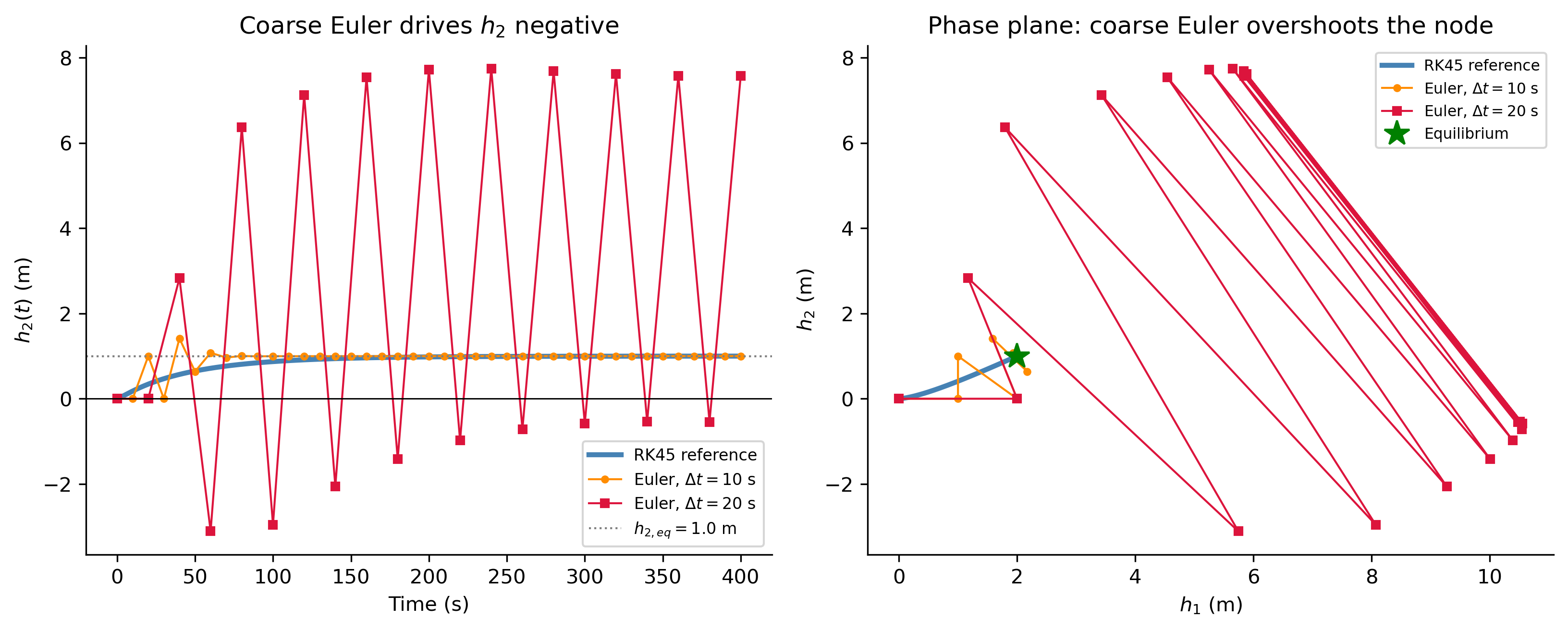
Because (Tanks–Nonlinear) has no closed-form solution, we must integrate it numerically — and this system is a good stress-test for numerical methods, because \(\sqrt{h_2}\) has an infinite slope at \(h_2=0\). Near the start of the simulation (both tanks empty), the local behavior is stiff enough that a coarse step size can produce not just an inaccurate answer, but a physically impossible one (a negative water height).

Show the code
def rhs_t(t, h):
    h1, h2 = max(h[0], -10), max(h[1], -10)
    Q12 = c12*np.sign(h1-h2)*np.sqrt(abs(h1-h2))
    Q2  = c2*np.sqrt(abs(h2)) * (1 if h2 >= 0 else -1)
    return [qin - Q12, Q12 - Q2]

t_final = 400
t_fine = np.linspace(0, t_final, 2000)
sol_ref = solve_ivp(rhs_t, (0, t_final), [0.0, 0.0], t_eval=t_fine, max_step=0.1)

def euler_fixed(dt):
    n = int(t_final/dt)
    h = np.zeros((n+1, 2))
    t = np.zeros(n+1)
    for i in range(n):
        h[i+1] = h[i] + dt*np.array(rhs_t(t[i], h[i]))
        t[i+1] = t[i] + dt
    return t, h

t_e10, h_e10 = euler_fixed(10.0)
t_e20, h_e20 = euler_fixed(20.0)

fig, axes = plt.subplots(1, 2, figsize=(11, 4.5))

axes[0].plot(sol_ref.t, sol_ref.y[1], color='steelblue', lw=2.5, label='RK45 reference')
axes[0].plot(t_e10, h_e10[:,1], 'o-', color='darkorange', ms=3, lw=1, label='Euler, $\\Delta t=10$ s')
axes[0].plot(t_e20, h_e20[:,1], 's-', color='crimson', ms=4, lw=1, label='Euler, $\\Delta t=20$ s')
axes[0].axhline(0, color='k', lw=0.7)
axes[0].axhline(h_eq_nl[1], color='gray', ls=':', lw=1, label=f'$h_{{2,eq}}={h_eq_nl[1]:.1f}$ m')
axes[0].set_xlabel('Time (s)'); axes[0].set_ylabel('$h_2(t)$ (m)')
axes[0].set_title('Coarse Euler drives $h_2$ negative')
axes[0].legend(fontsize=8)

axes[1].plot(sol_ref.y[0], sol_ref.y[1], color='steelblue', lw=2.5, label='RK45 reference')
axes[1].plot(h_e10[:,0], h_e10[:,1], 'o-', color='darkorange', ms=3, lw=1, label='Euler, $\\Delta t=10$ s')
axes[1].plot(h_e20[:,0], h_e20[:,1], 's-', color='crimson', ms=4, lw=1, label='Euler, $\\Delta t=20$ s')
axes[1].plot(h_eq_nl[0], h_eq_nl[1], 'g*', ms=13, label='Equilibrium', zorder=5)
axes[1].set_xlabel('$h_1$ (m)'); axes[1].set_ylabel('$h_2$ (m)')
axes[1].set_title('Phase plane: coarse Euler overshoots the node')
axes[1].legend(fontsize=7.5)

plt.tight_layout()
plt.show()
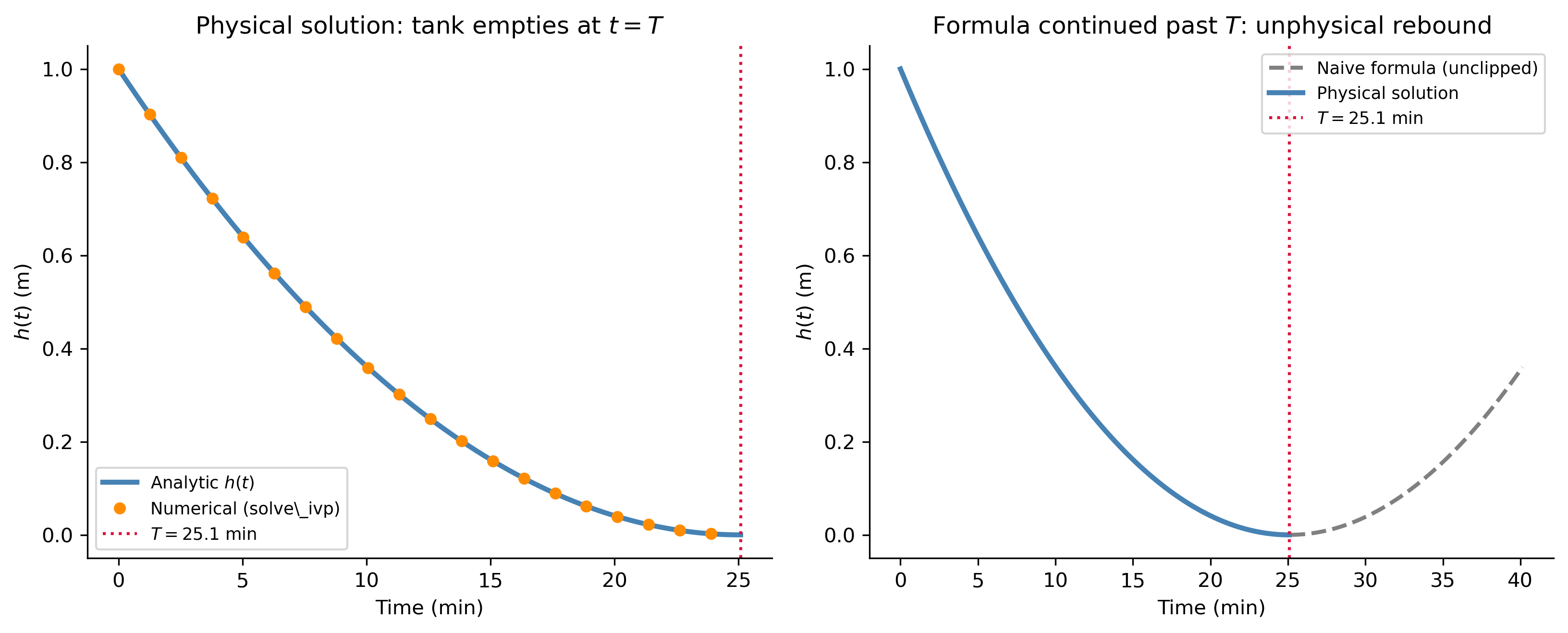
Figure 4: Same nonlinear tank system, starting empty. Left: \(h_2(t)\) under three methods — a fine RK45 reference (solve_ivp, effectively exact), fixed-step Euler with \(\Delta t=10\) s (visually indistinguishable from the reference), and Euler with \(\Delta t=20\) s (overshoots and drives \(h_2\) negative — an unphysical result). Right: the same comparison in the phase plane; the coarse-Euler trajectory spirals away from the true solution instead of settling smoothly onto the equilibrium node.
NoteWhy This Happens

Euler’s method takes a single linear step using the slope at the start of the interval. When \(h_2\) is small, \(d(\sqrt{h_2})/dh_2 = 1/(2\sqrt{h_2})\) is enormous, so the true solution curves sharply — a large step size badly misjudges how much \(h_2\) should change and can overshoot past zero into “negative water,” after which the (still-large) slope estimate overcorrects in the other direction, producing the oscillatory blow-up seen above. Halving the step size to \(\Delta t=10\) s is already enough to tame it here. This is exactly the kind of local-error analysis behind adaptive step-size control in solve_ivp, and a good reason to always sanity-check a numerical solution against the physics (can \(h_2\) actually be negative?).


Part 4 — Motion Through a Fluid: Stokes Drag vs. Quadratic Drag

Newton’s Second Law with Drag

An object of mass \(m\) falling through a fluid experiences gravity and a drag force opposing its motion. Which drag law applies depends on the Reynolds number \(Re\), a dimensionless ratio of inertial to viscous forces:

Regime Drag law Force ODE
\(Re \ll 1\) (Stokes / laminar) Linear in \(v\) \(F_d = 6\pi\mu r v\) \(m v' = mg - 6\pi\mu r\,v\)
\(Re \gg 1\) (form / turbulent) Quadratic in \(v\) \(F_d = \tfrac12\rho C_d A v^2\) \(m v' = mg - k v^2\)

Here \(\mu\) is the fluid’s dynamic viscosity, \(r\) the object’s radius, \(\rho\) the fluid density, \(C_d\) a drag coefficient, and \(A\) the object’s cross-sectional area. Both are first-order ODEs for \(v(t)\) — but one is linear and one is nonlinear, letting us directly compare techniques on the same physical problem.

Case 1: Stokes (Linear) Drag — a Settling Sphere

For a small sphere settling slowly through a viscous fluid (e.g., a steel ball bearing sinking in glycerin), \(mv' = mg - cv\) with \(c=6\pi\mu r\). This is the familiar linear first-order ODE from Notes 2: \[ \boxed{v(t) = v_{term}\left(1-e^{-t/\tau}\right)}, \qquad v_{term} = \frac{mg}{c}, \quad \tau = \frac{m}{c}. \]

Case 2: Quadratic (Form) Drag — a Skydiver

For a large, fast-moving object in air (a skydiver in free fall), the Reynolds number is huge and drag is quadratic: \(mv' = mg - kv^2\), which is nonlinear but still separable. Writing \(v_{term}^2 = mg/k\), \[ \frac{dv}{dt} = g\left(1 - \frac{v^2}{v_{term}^2}\right) \quad\Longrightarrow\quad \int \frac{dv}{1-(v/v_{term})^2} = \int g\,dt. \] The left integral is \(v_{term}\operatorname{artanh}(v/v_{term})\), so (with \(v(0)=0\)): \[ \boxed{v(t) = v_{term}\tanh\!\left(\frac{gt}{v_{term}}\right)}. \] Integrating once more gives the distance fallen, \[ x(t) = \frac{v_{term}^2}{g}\ln\!\left[\cosh\!\left(\frac{gt}{v_{term}}\right)\right]. \]

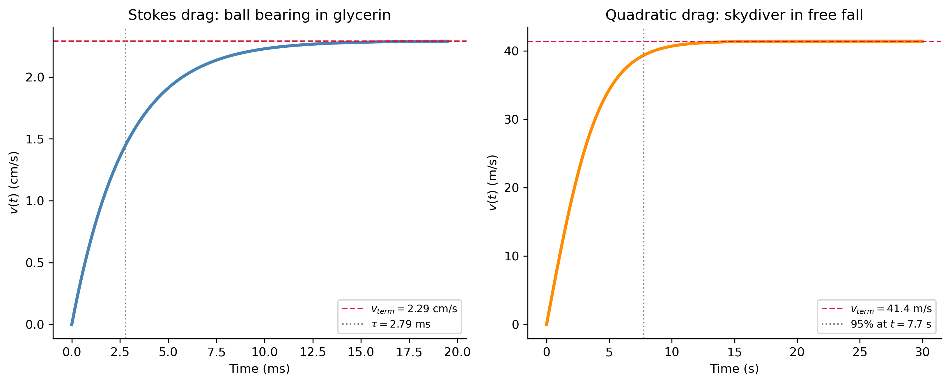
Both models describe an object approaching a terminal velocity, but the shape of the approach differs: \(1-e^{-t/\tau}\) has a constant relative decay rate, while \(\tanh\) approaches its asymptote with the same qualitative S-shaped saturation but arises from an entirely different (nonlinear) mechanism.

Show the code
g = 9.81

# ── Stokes drag: steel ball bearing in glycerin ──────────────
r_ball   = 1.5e-3      # m
rho_steel, rho_gly, mu = 7800.0, 1260.0, 1.4
m_ball   = (4/3)*np.pi*r_ball**3*rho_steel
Vol_ball = (4/3)*np.pi*r_ball**3
net_grav = m_ball*g - rho_gly*Vol_ball*g   # weight minus buoyancy
c_stokes = 6*np.pi*mu*r_ball
v_term_s = net_grav/c_stokes
tau_s    = m_ball/c_stokes
Re_s     = rho_gly*v_term_s*(2*r_ball)/mu
print(f"Stokes: v_term = {v_term_s*100:.2f} cm/s, tau = {tau_s*1e3:.2f} ms, Re = {Re_s:.3f}")

# ── Quadratic drag: skydiver ──────────────────────────────────
m_sky, rho_air, Cd_sky, Area = 75.0, 1.225, 1.0, 0.7
k_quad   = 0.5*rho_air*Cd_sky*Area
v_term_q = np.sqrt(m_sky*g/k_quad)
t95      = v_term_q/g*np.arctanh(0.95)
print(f"Quadratic: v_term = {v_term_q:.2f} m/s = {v_term_q*3.6:.0f} km/h, t95% = {t95:.2f} s")

fig, axes = plt.subplots(1, 2, figsize=(11, 4.5))

t_s = np.linspace(0, 7*tau_s, 300)
v_s = v_term_s*(1-np.exp(-t_s/tau_s))
axes[0].plot(t_s*1e3, v_s*100, color='steelblue', lw=2.5)
axes[0].axhline(v_term_s*100, color='crimson', ls='--', lw=1.2, label=f'$v_{{term}}={v_term_s*100:.2f}$ cm/s')
axes[0].axvline(tau_s*1e3, color='gray', ls=':', lw=1.2, label=f'$\\tau={tau_s*1e3:.2f}$ ms')
axes[0].set_xlabel('Time (ms)'); axes[0].set_ylabel('$v(t)$ (cm/s)')
axes[0].set_title('Stokes drag: ball bearing in glycerin')
axes[0].legend(fontsize=8.5)

t_q = np.linspace(0, 30, 300)
v_q = v_term_q*np.tanh(g*t_q/v_term_q)
axes[1].plot(t_q, v_q, color='darkorange', lw=2.5)
axes[1].axhline(v_term_q, color='crimson', ls='--', lw=1.2, label=f'$v_{{term}}={v_term_q:.1f}$ m/s')
axes[1].axvline(t95, color='gray', ls=':', lw=1.2, label=f'95% at $t={t95:.1f}$ s')
axes[1].set_xlabel('Time (s)'); axes[1].set_ylabel('$v(t)$ (m/s)')
axes[1].set_title('Quadratic drag: skydiver in free fall')
axes[1].legend(fontsize=8.5)

plt.tight_layout()
plt.show()
Stokes: v_term = 2.29 cm/s, tau = 2.79 ms, Re = 0.062
Quadratic: v_term = 41.43 m/s = 149 km/h, t95% = 7.74 s
Figure 5: Two drag regimes for the same Newton’s-second-law setup. Left: a 3 mm-diameter steel ball bearing settling in glycerin (\(Re\approx0.06\), Stokes regime) reaches terminal velocity in a few milliseconds (\(\tau=2.8\) ms). Right: a skydiver in free fall (\(Re\gg1\), quadratic-drag regime) reaches 95% of terminal velocity (\(\approx41.4\) m/s \(\approx149\) km/h) after about 7.7 s — the qualitative S-shape looks similar, but the underlying ODE, and the physical mechanism, are completely different.

Part 5 (Optional Capstone) — The Surge Tank and Laplace Transforms

Physical Setup

A surge tank is a vertical shaft added to a hydropower penstock (the pressurized pipe carrying water from a reservoir to a turbine) to absorb pressure transients. If a downstream valve closes suddenly, the moving column of water cannot stop instantly, and without a surge tank the resulting pressure spike (“water hammer”) could rupture the pipe. Instead, the water surges up into the tank and oscillates before settling to a new steady level. With appropriate linearization of the friction terms, the water-level deviation \(z(t)\) in the surge tank satisfies a linear, constant-coefficient, second-order ODE — structurally identical to the RLC circuit and the mass–spring–damper system studied elsewhere in this course: \[ \boxed{z'' + 2\zeta\omega_n\,z' + \omega_n^2\,z = \omega_n^2\,z_{ss}\,u(t),} \tag{Surge} \] where \(u(t)\) is the unit step function (modeling a valve closure at \(t=0\) that shifts the target level from \(0\) to \(z_{ss}\)), \(\omega_n\) is the natural surge frequency (set by the tank and tunnel geometry), and \(\zeta\) is a damping ratio (set by pipe friction).

Solving with the Laplace Transform

Taking the Laplace transform of (Surge) with zero initial conditions: \[ \left(s^2 + 2\zeta\omega_n s + \omega_n^2\right)Z(s) = \frac{\omega_n^2\,z_{ss}}{s} \quad\Longrightarrow\quad Z(s) = \frac{\omega_n^2\,z_{ss}}{s\left(s^2+2\zeta\omega_n s+\omega_n^2\right)}. \] Inverting (by partial fractions, exactly the underdamped case worked out for the RLC circuit and the DC motor) gives the classical underdamped step response: \[ \boxed{z(t) = z_{ss}\left[1 - \frac{e^{-\zeta\omega_n t}}{\sqrt{1-\zeta^2}}\sin(\omega_d t + \phi)\right]}, \qquad \omega_d = \omega_n\sqrt{1-\zeta^2}, \quad \phi = \arccos\zeta. \]

Show the code
t, s = sym.symbols('t s', positive=True)
zeta_s, wn_s, zss_s = sym.symbols('zeta omega_n z_ss', positive=True)

Zs = wn_s**2*zss_s/(s*(s**2 + 2*zeta_s*wn_s*s + wn_s**2))
z_of_t = sym.inverse_laplace_transform(Zs, s, t)
display(Math("Z(s) = " + sym.latex(Zs)))
display(Math("z(t) = " + sym.latex(sym.simplify(z_of_t))))

\(\displaystyle Z(s) = \frac{\omega_{n}^{2} z_{ss}}{s \left(\omega_{n}^{2} + 2 \omega_{n} s \zeta + s^{2}\right)}\)

\(\displaystyle z(t) = - \frac{z_{ss} \zeta e^{- \omega_{n} t \zeta} \sin{\left(\omega_{n} t \sqrt{1 - \zeta^{2}} \right)}}{\sqrt{1 - \zeta^{2}}} + z_{ss} - z_{ss} e^{- \omega_{n} t \zeta} \cos{\left(\omega_{n} t \sqrt{1 - \zeta^{2}} \right)}\)

For a lightly damped surge tank (\(\zeta=0.15\), \(\omega_n = 0.05\) rad/s, corresponding to a natural surge period of about two minutes) responding to a valve closure that raises the target level by \(z_{ss}=2\) m:

Show the code
zeta_v, wn_v, zss_v = 0.15, 0.05, 2.0
wd_v = wn_v*np.sqrt(1-zeta_v**2)
phi_v = np.arccos(zeta_v)
tp_v  = np.pi/wd_v
OS_v  = np.exp(-zeta_v*np.pi/np.sqrt(1-zeta_v**2))
ts_2pct = 4/(zeta_v*wn_v)
print(f"Peak time = {tp_v:.1f} s = {tp_v/60:.2f} min,  overshoot = {OS_v*100:.1f}%")
print(f"Peak level = {zss_v*(1+OS_v):.2f} m,  2%-settling time (est.) = {ts_2pct:.0f} s = {ts_2pct/60:.1f} min")

t_plot = np.linspace(0, 600, 1000)
z_t = zss_v*(1 - np.exp(-zeta_v*wn_v*t_plot)/np.sqrt(1-zeta_v**2)*np.sin(wd_v*t_plot + phi_v))

fig, ax = plt.subplots(figsize=(7.5, 4.5))
ax.plot(t_plot, z_t, color='steelblue', lw=2.5)
ax.axhline(zss_v, color='k', ls='--', lw=1, label=f'New steady level $z_{{ss}}={zss_v}$ m')
ax.plot(tp_v, zss_v*(1+OS_v), 'ro', ms=7, zorder=5,
        label=f'Peak: {zss_v*(1+OS_v):.2f} m at $t={tp_v:.0f}$ s')
ax.fill_between(t_plot, zss_v*0.98, zss_v*1.02, color='gray', alpha=0.15, label='$\\pm 2\\%$ band')
ax.set_xlabel('Time (s)'); ax.set_ylabel('Surge level $z(t)$ (m)')
ax.set_title('Surge-tank oscillation following a valve closure')
ax.legend(fontsize=8.5)
plt.tight_layout()
plt.show()

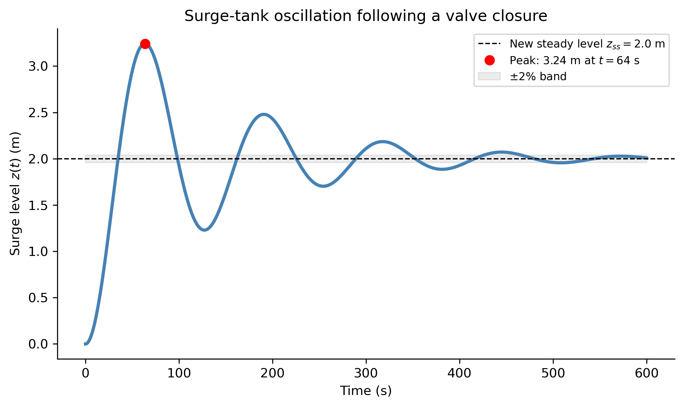
Peak time = 63.6 s = 1.06 min,  overshoot = 62.1%
Peak level = 3.24 m,  2%-settling time (est.) = 533 s = 8.9 min
Figure 6: Surge tank step response after a sudden valve closure (\(\zeta=0.15\), \(\omega_n=0.05\) rad/s, \(z_{ss}=2\) m). The level overshoots the new steady value by about 62% before oscillating (period \(\approx 2.1\) min) toward equilibrium. Light damping like this is exactly why real surge tanks add extra throttling to increase \(\zeta\) and tame the overshoot.
TipLooking Ahead: Laplace Transforms

The surge tank is the fluid-dynamics twin of the driven RLC circuit and the forced mass–spring–damper: same governing ODE, same Laplace-transform solution technique, same vocabulary of natural frequency, damping ratio, peak overshoot, and settling time. If you can solve one of these three problems with Laplace transforms, you can solve all of them — only the physical meaning of \(\omega_n\), \(\zeta\), and \(z_{ss}\) changes.


Connecting the Fluid-Dynamics Applications

Draining tank Coupled tanks (linear) Coupled tanks (nonlinear) Drag Surge tank
ODE type 1st-order, nonlinear (separable) 1st-order linear system 1st-order nonlinear system 1st-order, linear or nonlinear 2nd-order linear
Course topic Notes 2 Chapter 3 (systems) Chapter 3 + Numerical Methods Notes 2 Laplace transforms
Key parameter Drain time \(T=2\sqrt{h_0}/k\) Eigenvalues of \(A\) Eigenvalues of Jacobian Time constant \(\tau\) or \(v_{term}\) \(\omega_n,\ \zeta\)
Long-term behavior Reaches 0 in finite time Stable node (no oscillation) Locally stable node Approaches \(v_{term}\) Damped oscillation
Engineering relevance Tank sizing, batch processes Reservoir/process networks Realistic valve networks Sedimentation, free fall, HVAC Hydropower, water hammer
TipThe Analogy, Extended

The hydraulic–electrical analogy from Part 2 extends naturally to mechanics as well — every linear storage-and-dissipation system in this course (RC/RLC circuits in Topics 6, the spring–mass–damper in Topics 5, and the tank networks here) is governed by the same handful of ODE structures:

Fluid Electrical Mechanical
Height \(h\) Voltage \(V\) Displacement \(x\)
Flow rate \(Q\) Current \(I\) Velocity \(x'\)
Tank area \(A\) Capacitance \(C\) \(1/k\) (inverse spring constant)
Valve resistance \(R\) Resistance \(R\) Damping \(\gamma\)
(no direct analog) Inductance \(L\) Mass \(m\)

Notice the tank network has no analog of \(L\) or \(m\) — nothing in it stores inertia — which is precisely why coupled tanks can only settle monotonically to equilibrium, while RLC circuits and mass–spring systems can ring. The surge tank in Part 5 is the exception: the momentum of the moving water column in the connecting tunnel does act like an inductor/mass, which is exactly what makes surge-tank oscillations possible in the first place.


Relevant Videos

Torricelli’s Law:


References

Show the code
import sys
print("Python version:", sys.version)
print('\n'.join(f'{m.__name__}=={m.__version__}' for m in globals().values() if getattr(m, '__version__', None)))
Python version: 3.14.4 | packaged by conda-forge | (main, Apr  8 2026, 02:33:53) [Clang 20.1.8 ]
numpy==2.4.3
sympy==1.14.0
matplotlib==3.10.8

Reuse

CC BY-NC-SA 4.0