Thermodynamics and Heat Transfer: ODE Applications

Applications to Engineering and Physics

Show the code
import numpy as np
import sympy as sym
import matplotlib as mpl
import matplotlib.pyplot as plt
from scipy.integrate import solve_ivp
from IPython.display import Math, display
mpl.rcParams['figure.dpi'] = 150
mpl.rcParams['axes.spines.top'] = False
mpl.rcParams['axes.spines.right'] = False

Thermodynamics and heat transfer are, in a precise sense, an ODE laboratory: nearly every governing law in the subject — Newton’s law of cooling, the Stefan–Boltzmann radiation law, and the first law of thermodynamics applied to a piston-cylinder — is itself a first-order differential equation, or gives rise to one the moment a system is allowed to evolve in time. This makes heat transfer an unusually rich source of applications for a differential equations course, since it touches every major topic in (Logan 2015): first-order linear equations, systems of linear equations, Laplace transforms, nonlinear equations, and numerical methods all appear naturally, often within the same physical problem. This section develops six progressively richer applications, plus one enrichment topic for the mechanical engineers in the room:

  1. Newton’s law of cooling — a first-order linear ODE derived from a lumped energy balance, the thermal counterpart of Notes 2.
  2. The thermal–electrical analogy — showing that thermal circuits obey the same mathematics as the RC circuits of Topics 6.
  3. Multi-node thermal networks — coupled bodies exchanging heat, a system of linear ODEs whose eigenvalues are physical equilibration rates.
  4. Periodic ambient forcing — a forced linear ODE solved by Laplace transform methods, producing phase lag and amplitude attenuation exactly as in the RC low-pass filter.
  5. Nonlinear radiative cooling — the Stefan–Boltzmann law gives a genuinely nonlinear separable ODE with a transcendental closed-form solution.
  6. Combined-mode heat transfer and numerical methods — convection and radiation acting together admit no closed form, motivating Euler, Heun, and Runge–Kutta methods.
  7. Bonus — the polytropic piston–cylinder — the first law of thermodynamics, the ideal gas law, and Newton’s law of cooling combine into a single first-order linear ODE that unifies adiabatic and non-adiabatic gas processes.

Part 1 — Newton’s Law of Cooling: Lumped-Capacitance Heat Transfer

Physical Setup and the Energy Balance

Consider a body — a hot bearing, a beverage, a heat sink, a thermocouple bead — with mass \(m\), specific heat \(c\), and (for now) spatially uniform internal temperature \(T(t)\), immersed in a large surrounding environment held at constant temperature \(T_{env}\). Heat leaves the body by convection at its surface (area \(A\)), governed by Newton’s law of cooling: the convective heat flux is proportional to the temperature difference between the surface and the environment, with proportionality constant \(h\) (the convective heat transfer coefficient, \(\text{W}/\text{m}^2\text{K}\)).

A first-law (conservation of energy) balance on the body states that the rate of change of its internal (thermal) energy equals the rate at which heat leaves through its surface: \[ \underbrace{mc\,\frac{dT}{dt}}_{\text{rate of change of internal energy}} = \underbrace{-hA\big(T - T_{env}\big)}_{\text{rate of heat loss by convection}}. \] Dividing through by \(mc\): \[ \boxed{\frac{dT}{dt} = -k\big(T - T_{env}\big),} \qquad k = \frac{hA}{mc}. \tag{NC} \] This is exactly the first-order linear ODE of Notes 2 — indeed it is the same equation as (RC) in Topics 6, with \(T\) playing the role of \(V_C\). The constant \(k\) has units of inverse time; \(\tau = 1/k\) is the thermal time constant.

NoteValidity of the Lumped-Capacitance Model

Treating the body as having one spatially-uniform temperature \(T(t)\) — the lumped-capacitance approximation — is an idealization. It is justified when internal conduction is much faster than surface convection, i.e., when the Biot number \[ \text{Bi} = \frac{hL_c}{k_{\text{material}}} \ll 1 \quad (\text{typically } \text{Bi} < 0.1) \] is small, where \(L_c = V/A\) is a characteristic length and \(k_{\text{material}}\) is the thermal conductivity of the body (not to be confused with the rate constant \(k\) above). Physically: small, highly conductive bodies (a thermocouple bead, a small metal part) satisfy this well; large or poorly-conductive bodies (a roast in an oven, a brick wall) do not, and require the heat equation (a PDE) rather than a single ODE.

Solution and the Thermal Time Constant

Equation (NC) is separable (or solved directly by the integrating factor of Notes 2). With \(T(0) = T_0\): \[ \boxed{T(t) = T_{env} + (T_0 - T_{env})\,e^{-t/\tau},} \qquad \tau = \frac{1}{k} = \frac{mc}{hA}. \] The body approaches ambient temperature exponentially, reaching \(63.2\%\) of the total temperature change at \(t=\tau\) and essentially equilibrating (\(>99\%\)) by \(t = 5\tau\) — precisely the same “charge/discharge” behavior as the RC circuit’s step response.

Thermal Time Constants in Practice

The time constant \(\tau = mc/(hA)\) depends on the body’s mass, material, geometry, and the strength of convection at its surface. Compact, lightweight objects in strong forced convection have short time constants (seconds); larger objects in still air have much longer ones (tens of minutes).

Show the code
examples = [
    ("Steel bearing, still air",      0.50, 200.0, 25.0, 15.0, 0.05, 500.0),
    ("Coffee cup, still air",         0.30,  90.0, 22.0,  8.0, 0.02, 4200.0),
    ("CPU heat sink, forced air",     0.05,  85.0, 25.0, 40.0, 0.01, 900.0),
]
# columns: label, m (kg), T0 (C), Tenv (C), h (W/m2K), A (m^2), c (J/kgK)

t_plot = np.linspace(0, 1800, 500)
colors = ['steelblue', 'darkorange', 'crimson']

fig, ax = plt.subplots(figsize=(8, 4.5))
for (lbl, m, T0, Tenv, h, A, c), color in zip(examples, colors):
    k = h*A/(m*c)
    tau = 1/k
    T = Tenv + (T0 - Tenv)*np.exp(-k*t_plot)
    ax.plot(t_plot, T, color=color, lw=2.2, label=f'{lbl} ($\\tau={tau:.0f}$ s)')
    ax.axhline(Tenv, color='gray', lw=0.5, ls=':')

ax.set_xlabel('$t$ (s)'); ax.set_ylabel('Temperature (°C)')
ax.set_title("Newton's law of cooling: $T(t) = T_{env} + (T_0-T_{env})e^{-t/\\tau}$")
ax.legend(fontsize=8.5)
plt.tight_layout()
plt.show()
Figure 1: Newton’s law of cooling for three lumped bodies with different mass, specific heat, and convective conditions. Each curve decays exponentially toward \(T_{env}\) with its own thermal time constant \(\tau = mc/(hA)\); smaller, better-cooled bodies (e.g. a forced-air heat sink) equilibrate far faster than a coffee cup in still air.
TipMeasuring \(h\) from Data

Just as the spring constant \(k\) can be measured from a static elongation (Topics 5), the convective coefficient \(h\) can be estimated from a measured cooling curve: rearranging (NC), \[ \ln\!\big(T(t) - T_{env}\big) = \ln(T_0 - T_{env}) - kt, \] so a plot of \(\ln(T - T_{env})\) against \(t\) should be a straight line of slope \(-k = -hA/(mc)\). This linear-regression technique — fitting a first-order linear ODE’s solution to data — is a common step in experimental heat-transfer courses and a nice preview of parameter estimation.


Part 2 — The Thermal–Electrical Analogy

The Correspondence

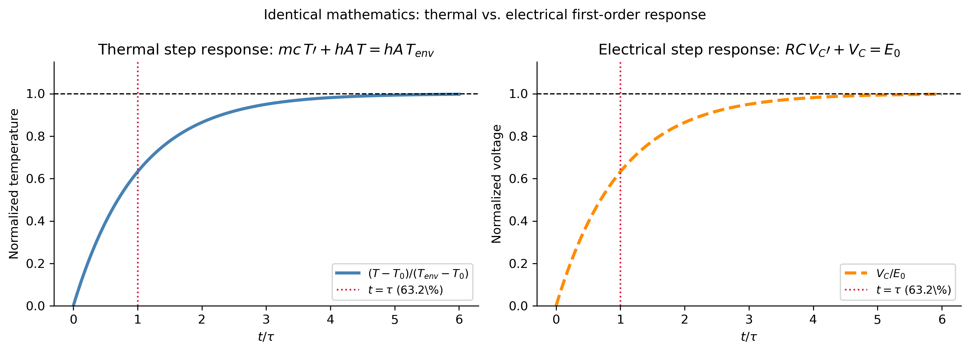
Comparing (NC) to the RC circuit equation of Topics 6, \[ \frac{dT}{dt} + kT = kT_{env} \qquad\text{(thermal)} \] \[ RC\,\frac{dV_C}{dt} + V_C = V_{in}(t) \qquad\text{(electrical, rearranged)} \] reveals that a lumped thermal system and an RC circuit obey identical mathematics. The correspondence extends to multi-node networks (Part 3) and is summarized below:

Thermal Symbol Electrical Symbol
Temperature \(T\) Voltage \(V\)
Heat flow rate \(\dot Q\) Current \(I\)
Thermal resistance \(R_t = \dfrac{1}{hA}\) Resistance \(R\)
Thermal capacitance \(C_t = mc\) Capacitance \(C\)
Thermal time constant \(\tau = R_tC_t = \dfrac{mc}{hA}\) Time constant \(\tau = RC\)
Ambient/source temperature \(T_{env}\) Source voltage \(V_{in}\)
Heat stored \(mcT\) Charge stored \(Q = CV\)
TipWhy the Analogy Matters

The analogy is not a coincidence — both systems are governed by a single conserved quantity (energy, charge) flowing through a resistance in response to a potential difference (temperature difference, voltage difference), accumulating in a capacity (thermal mass, capacitor). This means every technique from Topics 6 — time constants, step response, frequency response — transfers immediately to thermal systems, and vice versa. Thermal engineers routinely draw thermal resistance networks using the same circuit diagrams (resistors and capacitors) that electrical engineers use, and simulate them with electrical-circuit software (SPICE) — this is precisely why the analogy is taught in both disciplines.

Show the code
tau = 1.0
t_plot = np.linspace(0, 6, 400)
resp = 1 - np.exp(-t_plot/tau)

fig, axes = plt.subplots(1, 2, figsize=(11, 4))

axes[0].plot(t_plot, resp, color='steelblue', lw=2.5, label='$(T-T_0)/(T_{env}-T_0)$')
axes[0].axhline(1.0, color='k', ls='--', lw=1)
axes[0].axvline(1.0, color='crimson', ls=':', lw=1.3, label=r'$t=\tau$ (63.2\%)')
axes[0].set_xlabel('$t/\\tau$'); axes[0].set_ylabel('Normalized temperature')
axes[0].set_title(r'Thermal step response: $mc\,T\prime + hA\,T = hA\,T_{env}$')
axes[0].legend(fontsize=9); axes[0].set_ylim(0, 1.15)

axes[1].plot(t_plot, resp, color='darkorange', lw=2.5, ls='--', label='$V_C/E_0$')
axes[1].axhline(1.0, color='k', ls='--', lw=1)
axes[1].axvline(1.0, color='crimson', ls=':', lw=1.3, label=r'$t=\tau$ (63.2\%)')
axes[1].set_xlabel('$t/\\tau$'); axes[1].set_ylabel('Normalized voltage')
axes[1].set_title(r'Electrical step response: $RC\,V_C\prime + V_C = E_0$')
axes[1].legend(fontsize=9); axes[1].set_ylim(0, 1.15)

plt.suptitle('Identical mathematics: thermal vs. electrical first-order response', fontsize=11)
plt.tight_layout()
plt.show()
Figure 2: The thermal–electrical analogy. A lumped thermal system (left) and an RC circuit (right) obey identical first-order linear ODEs. Both curves show the identical dimensionless step response \(1-e^{-t/\tau}\) — a body heated from \(T_{env}\) toward a fixed boundary temperature (left) is mathematically the same problem as a capacitor charging toward a battery voltage (right).

Part 3 — Multi-Node Thermal Networks: Systems of Linear ODEs

Two Coupled Bodies

Real thermal systems rarely consist of a single lumped mass. Consider a CPU chip (temperature \(T_1\)) mounted on a heat sink (temperature \(T_2\)), both exchanging heat with each other and with a common ambient temperature \(T_{env}\). Writing a first-law balance for each node: \[ \frac{dT_1}{dt} = -k_{1,env}(T_1 - T_{env}) - k_{12}(T_1 - T_2), \] \[ \frac{dT_2}{dt} = -k_{2,env}(T_2 - T_{env}) - k_{12}(T_2 - T_1), \] where \(k_{1,env}, k_{2,env}\) describe each node’s own convective loss to ambient, and \(k_{12}\) describes conductive/contact coupling between the two nodes. In matrix form, \(\mathbf{T} = (T_1, T_2)^\top\) satisfies: \[ \boxed{\mathbf{T}' = A\mathbf{T} + \mathbf{b}}, \qquad A = \begin{pmatrix} -(k_{1,env}+k_{12}) & k_{12} \\ k_{12} & -(k_{2,env}+k_{12}) \end{pmatrix}, \quad \mathbf{b} = \begin{pmatrix} k_{1,env}T_{env} \\ k_{2,env}T_{env} \end{pmatrix}. \] This is precisely a linear system of ODEs (Chapter 3), with a constant, nonhomogeneous forcing vector \(\mathbf b\).

ImportantEigenvalues as Physical Equilibration Rates

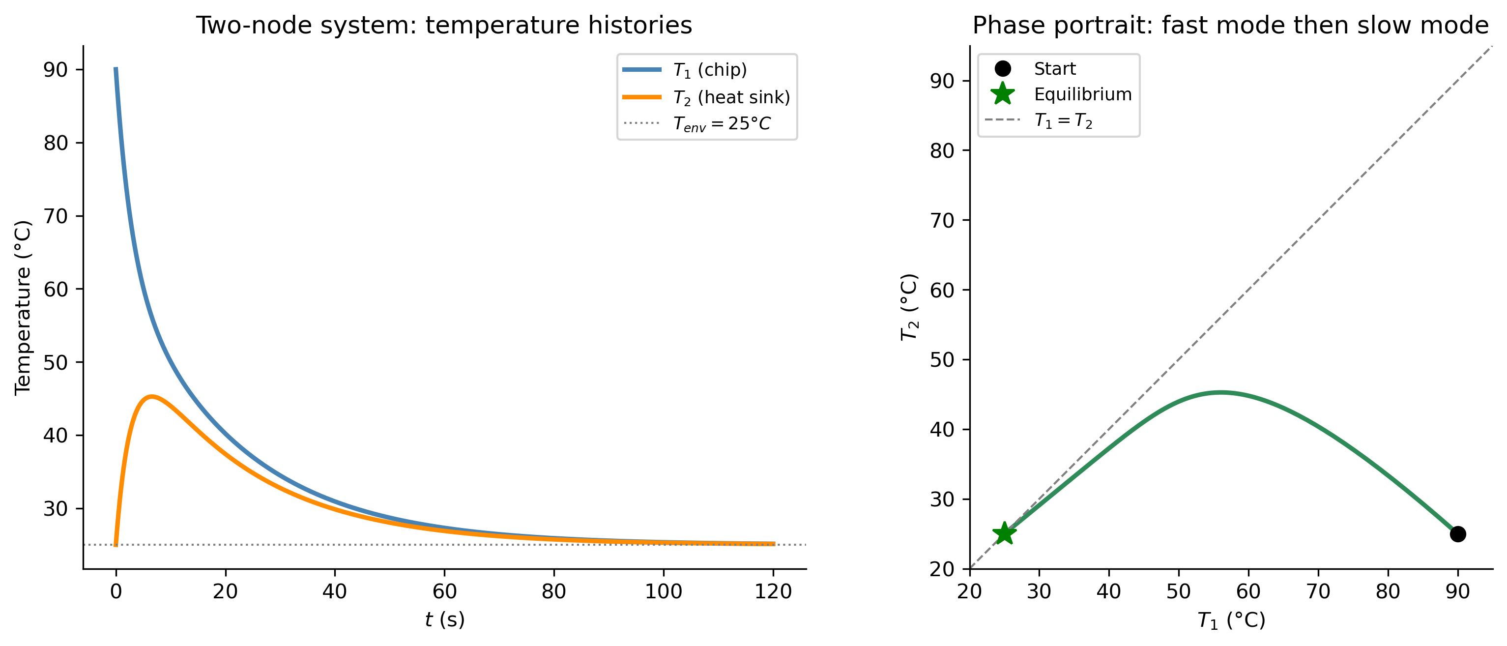
The eigenvalues \(\lambda_1, \lambda_2\) of \(A\) are both real and negative (the system is thermally stable — heat only flows from hot to cold). They have direct physical meaning: the corresponding eigenvectors are the thermal modes of the coupled system. Typically one eigenvalue is much more negative than the other, giving:

  • a fast mode (\(|\lambda|\) large) in which the chip and heat sink rapidly equilibrate with each other (governed mainly by \(k_{12}\));
  • a slow mode (\(|\lambda|\) small) in which the combined chip+sink system slowly equilibrates with the ambient environment.

This is exactly analogous to normal modes in coupled mechanical oscillators, and it is why a heat sink stabilizes chip temperature quickly even though the whole assembly takes much longer to reach room temperature.

Show the code
k1env, k2env, k12 = 0.02, 0.08, 0.15   # 1/s
Tenv = 25.0

A_mat = np.array([[-(k1env+k12),  k12],
                   [k12,          -(k2env+k12)]])
b_vec = np.array([k1env*Tenv, k2env*Tenv])

eigvals, eigvecs = np.linalg.eig(A_mat)
print("Eigenvalues (1/s):", eigvals)
print("Time constants (s):", -1/eigvals)

def rhs(t, T):
    return A_mat @ T + b_vec

T0 = np.array([90.0, 25.0])
t_plot = np.linspace(0, 120, 500)
sol = solve_ivp(rhs, (0, 120), T0, t_eval=t_plot, max_step=0.1)

fig, axes = plt.subplots(1, 2, figsize=(11, 4.5))

axes[0].plot(sol.t, sol.y[0], color='steelblue', lw=2.2, label='$T_1$ (chip)')
axes[0].plot(sol.t, sol.y[1], color='darkorange', lw=2.2, label='$T_2$ (heat sink)')
axes[0].axhline(Tenv, color='gray', ls=':', lw=1, label='$T_{env}=25°C$')
axes[0].set_xlabel('$t$ (s)'); axes[0].set_ylabel('Temperature (°C)')
axes[0].set_title('Two-node system: temperature histories')
axes[0].legend(fontsize=8.5)

axes[1].plot(sol.y[0], sol.y[1], color='seagreen', lw=2.2)
axes[1].plot(T0[0], T0[1], 'ko', markersize=7, label='Start', zorder=5)
axes[1].plot(Tenv, Tenv, 'g*', markersize=12, label='Equilibrium', zorder=5)
lims = [20, 95]
axes[1].plot(lims, lims, color='gray', ls='--', lw=1, label='$T_1=T_2$')
axes[1].set_xlabel('$T_1$ (°C)'); axes[1].set_ylabel('$T_2$ (°C)')
axes[1].set_title('Phase portrait: fast mode then slow mode')
axes[1].legend(fontsize=8.5); axes[1].set_xlim(lims); axes[1].set_ylim(lims)
axes[1].set_aspect('equal')

plt.tight_layout()
plt.show()
Eigenvalues (1/s): [-0.04702941 -0.35297059]
Time constants (s): [21.26328828  2.83309726]
Figure 3: Two-node thermal network: a chip (\(T_1\)) on a heat sink (\(T_2\)), both losing heat to ambient. Left: temperature histories starting from a hot chip and room-temperature heat sink — the two temperatures merge quickly (fast mode) and then decay together toward ambient (slow mode). Right: phase portrait \((T_1,T_2)\); the trajectory first moves toward the diagonal \(T_1=T_2\) (fast mode) before sliding down the diagonal toward equilibrium (slow mode).

The printed eigenvalues confirm the two-timescale structure: one eigenvalue is roughly \(7\times\) larger in magnitude than the other, giving a fast chip–sink equilibration followed by a much slower combined decay to ambient — exactly the qualitative picture described above. This construction generalizes directly to an \(n\)-node network (e.g., several rooms in a building, or a discretized rod), where it becomes the finite-difference approximation to the heat equation — a natural preview of PDE methods for students who continue past this course.


Part 4 — Periodic Ambient Forcing and the Laplace Transform

Setup

Suppose the ambient temperature itself varies periodically — a day/night cycle, a periodically cycling furnace, or a machine with a periodic heat load: \[ \frac{dT}{dt} + kT = k\,T_{env}(t), \qquad T_{env}(t) = T_0 + A_0\sin(\omega t). \tag{PF} \] This is a forced first-order linear ODE with sinusoidal forcing — an ideal candidate for the Laplace transform methods of the course, and structurally identical to a sinusoidally-driven RC circuit.

Solution by Laplace Transform

Taking the Laplace transform of (PF) with \(T(0)=T_0\) (so that the body starts at the mean ambient temperature) and using \(\mathcal{L}\{\sin\omega t\} = \omega/(s^2+\omega^2)\): \[ sX(s) - T_0 + kX(s) = k\left[\frac{T_0}{s} + \frac{A_0\omega}{s^2+\omega^2}\right], \qquad X(s) = \mathcal{L}\{T(t)\}. \] Solving for \(X(s)\) and performing the partial fraction decomposition (the transient term decays like \(e^{-kt}\) and is omitted here since we are interested in the long-time steady-state response), the particular/steady-state solution is: \[ \boxed{T_{ss}(t) = T_0 + A_0\,G(\omega)\sin(\omega t - \phi)}, \qquad G(\omega) = \frac{1}{\sqrt{1+(\omega/k)^2}}, \qquad \phi = \arctan\!\left(\frac{\omega}{k}\right). \]

TipThe Same Transfer Function as the RC Filter

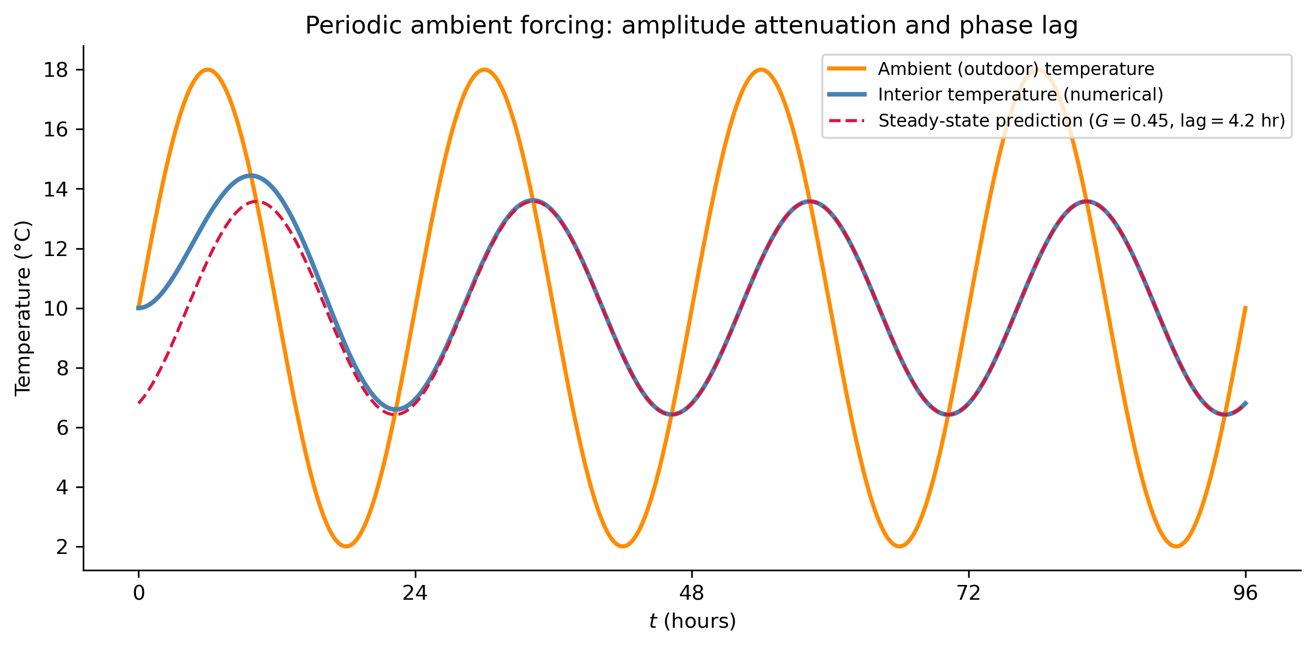
Compare \(G(\omega)\) above to the RC low-pass filter’s amplitude ratio from Topics 6, \(|H(\omega)| = 1/\sqrt{1+(\omega\tau)^2}\) with \(\tau = 1/k\)they are identical. A thermal system responding to a periodic ambient temperature is a low-pass filter: slow (low-frequency) ambient swings pass through nearly unattenuated (\(G\approx 1\) when \(\omega \ll k\)), while fast swings are strongly damped (\(G\to 0\) as \(\omega \to \infty\)) and phase-lagged. This is why a building’s interior temperature lags the outdoor daily cycle by several hours and swings by a much smaller amplitude than the outdoor air — the building’s thermal mass acts as a low-pass filter on the daily temperature wave.

Show the code
k = 2*np.pi/48      # 1/hr; thermal time constant tau = 1/k ~ 7.64 hr
T0mean = 10.0        # deg C, mean ambient
A0 = 8.0             # deg C, ambient swing amplitude
omega = 2*np.pi/24   # 1/hr, 24-hour period

def rhs(t, T):
    Tenv = T0mean + A0*np.sin(omega*t)
    return -k*(T - Tenv)

t_plot = np.linspace(0, 96, 700)
sol = solve_ivp(rhs, (0, 96), [T0mean], t_eval=t_plot, max_step=0.05)

G = 1/np.sqrt(1 + (omega/k)**2)
phi = np.arctan(omega/k)
print(f"Amplitude ratio G = {G:.3f},  phase lag = {phi:.3f} rad = {phi/omega:.2f} hr")

Tenv_plot = T0mean + A0*np.sin(omega*t_plot)
T_ss = T0mean + A0*G*np.sin(omega*t_plot - phi)

fig, ax = plt.subplots(figsize=(9, 4.5))
ax.plot(t_plot, Tenv_plot, color='darkorange', lw=2, label='Ambient (outdoor) temperature')
ax.plot(sol.t, sol.y[0], color='steelblue', lw=2.2, label='Interior temperature (numerical)')
ax.plot(t_plot, T_ss, color='crimson', lw=1.5, ls='--',
        label=f'Steady-state prediction ($G={G:.2f}$, lag$={phi/omega:.1f}$ hr)')
ax.set_xlabel('$t$ (hours)'); ax.set_ylabel('Temperature (°C)')
ax.set_title('Periodic ambient forcing: amplitude attenuation and phase lag')
ax.legend(fontsize=8.5)
ax.set_xticks([0, 24, 48, 72, 96])
plt.tight_layout()
plt.show()
Amplitude ratio G = 0.447,  phase lag = 1.107 rad = 4.23 hr
Figure 4: A thermally massive interior (\(k=2\pi/48\ \mathrm{hr}^{-1}\), i.e. \(\tau\approx 7.6\) hr) responding to a 24-hour ambient temperature cycle. The numerical solution (solid) settles onto the analytic steady-state response (dashed) derived by Laplace transform: the interior temperature swings with smaller amplitude (\(G(\omega)\approx 0.45\)) and lags the outdoor peak by about 4.2 hours (\(\phi/\omega\)).

Part 5 — Nonlinear Radiative Cooling: The Stefan–Boltzmann Law

The Nonlinear ODE

At high temperatures, heat loss by thermal radiation dominates over convection. The Stefan–Boltzmann law gives the radiative heat flux as proportional to \(T^4 - T_{env}^4\) (both temperatures in Kelvin), so the energy balance becomes: \[ mc\,\frac{dT}{dt} = -\varepsilon\sigma A\big(T^4 - T_{env}^4\big), \] where \(\varepsilon\in(0,1]\) is the surface emissivity and \(\sigma = 5.670\times10^{-8}\ \text{W}/(\text{m}^2\text{K}^4)\) is the Stefan–Boltzmann constant. Writing \(a = \varepsilon\sigma A/(mc)\): \[ \boxed{\frac{dT}{dt} = -a\big(T^4 - T_{env}^4\big).} \tag{RAD} \] Unlike Newton’s law of cooling, this equation is nonlinear in \(T\) — the right-hand side is a quartic, not a linear function of \(T\).

A Genuine Closed-Form Solution

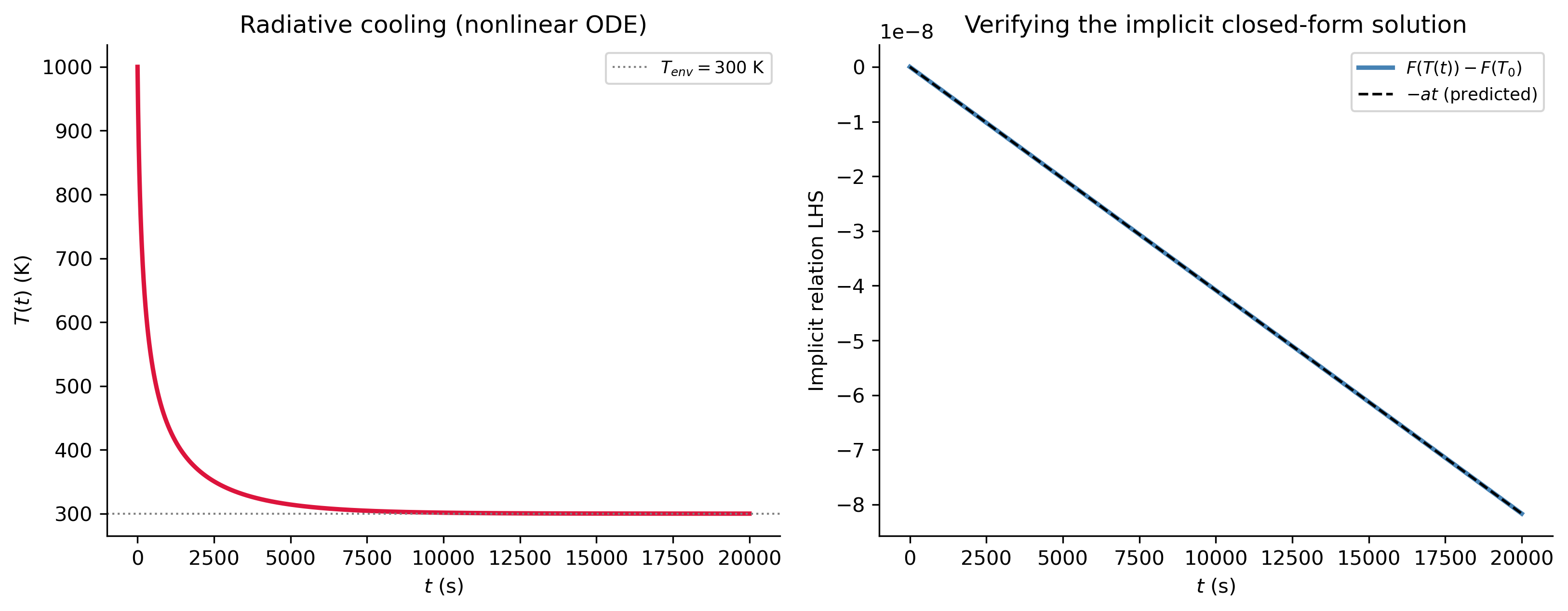
Equation (RAD) is separable. Writing \(b = T_{env}\) and factoring \(T^4 - b^4 = (T-b)(T+b)(T^2+b^2)\), the partial fraction decomposition gives: \[ \int \frac{dT}{T^4-b^4} = \frac{1}{4b^3}\ln\left|\frac{T-b}{T+b}\right| - \frac{1}{2b^3}\arctan\!\left(\frac{T}{b}\right) + C. \] Applying this to (RAD) and using \(T(0) = T_0\) gives the implicit closed-form solution: \[ \left[\frac{1}{4b^3}\ln\left|\frac{T-b}{T+b}\right| - \frac{1}{2b^3}\arctan\!\left(\frac{T}{b}\right)\right]_{T_0}^{T(t)} = -at. \] This is a genuine, exact solution — but it is transcendental in \(T\): there is no way to solve for \(T(t)\) explicitly. This is a valuable lesson for students: “solvable in closed form” for a nonlinear ODE often means implicitly solvable, and numerical methods (Part 6) remain the practical tool even when an exact solution exists on paper.

Show the code
sigma_SB = 5.670374419e-8
eps = 0.9
A_area = 0.02   # m^2
m_mass = 0.5    # kg
c_spec = 500.0  # J/(kg K)
Tenv_K = 300.0  # K
T0_K   = 1000.0 # K

a_rad = eps*sigma_SB*A_area/(m_mass*c_spec)

def rad_rhs(t, T):
    return -a_rad*(T**4 - Tenv_K**4)

t_plot = np.linspace(0, 20000, 2000)
sol = solve_ivp(rad_rhs, (0, 20000), [T0_K], t_eval=t_plot, max_step=5.0, rtol=1e-10, atol=1e-8)
T_num = sol.y[0]

b_K = Tenv_K
def F_implicit(T):
    return (1/(4*b_K**3))*np.log(np.abs((T-b_K)/(T+b_K))) - (1/(2*b_K**3))*np.arctan(T/b_K)

C0 = F_implicit(T0_K)
lhs_check = F_implicit(T_num) - C0

fig, axes = plt.subplots(1, 2, figsize=(11, 4.5))

axes[0].plot(t_plot, T_num, color='crimson', lw=2.2)
axes[0].axhline(Tenv_K, color='gray', ls=':', lw=1, label='$T_{env}=300$ K')
axes[0].set_xlabel('$t$ (s)'); axes[0].set_ylabel('$T(t)$ (K)')
axes[0].set_title('Radiative cooling (nonlinear ODE)')
axes[0].legend(fontsize=8.5)

axes[1].plot(t_plot, lhs_check, color='steelblue', lw=2.2, label='$F(T(t))-F(T_0)$')
axes[1].plot(t_plot, -a_rad*t_plot, color='k', ls='--', lw=1.3, label='$-at$ (predicted)')
axes[1].set_xlabel('$t$ (s)'); axes[1].set_ylabel('Implicit relation LHS')
axes[1].set_title('Verifying the implicit closed-form solution')
axes[1].legend(fontsize=8.5)

plt.tight_layout()
plt.show()
Figure 5: Radiative-only cooling of a small object from 1000 K to ambient (300 K), governed by the nonlinear Stefan–Boltzmann ODE. Left: the numerical solution \(T(t)\), which cools very rapidly while far from equilibrium (since the \(T^4\) term is huge) and very slowly as it approaches \(T_{env}\). Right: verification of the implicit closed-form solution — plotting the left-hand side function of \(T(t)\) against \(t\) produces a perfectly straight line of slope \(-a\), confirming the exact solution derived above.
NoteRadiation vs. Convection: Why High-Temperature Systems Behave Differently

Because radiative loss scales as \(T^4-T_{env}^4\) rather than \(T-T_{env}\), a body far above ambient cools much faster, relative to its temperature excess, than Newton’s law of cooling would predict — and the cooling rate falls off sharply as \(T\) approaches \(T_{env}\) (where \(T^4-T_{env}^4 \approx 4T_{env}^3(T-T_{env})\), recovering an effective linear law close to equilibrium). This is why furnace and spacecraft thermal design must use the nonlinear radiative law, while near-room-temperature problems (Parts 1–4) are well approximated by the linear model.


Part 6 — Combined-Mode Heat Transfer and Numerical Methods

An ODE With No Closed Form

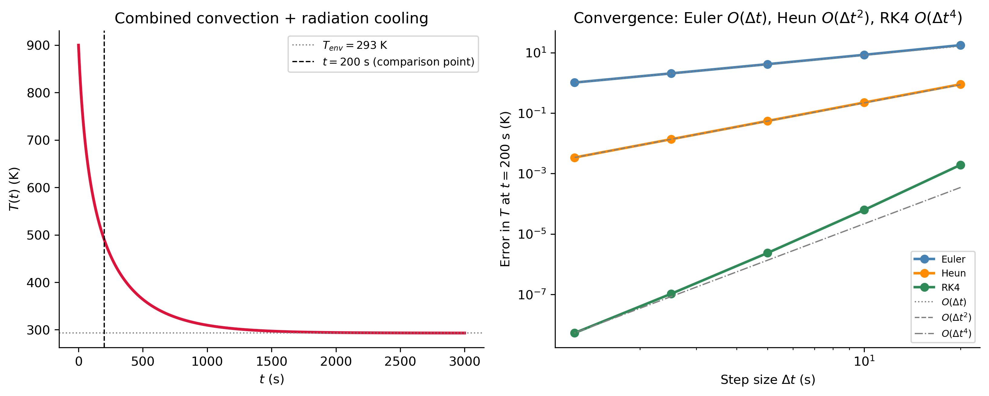
In practice, a hot object loses heat by both convection and radiation simultaneously: \[ mc\,\frac{dT}{dt} = -hA(T-T_{env}) - \varepsilon\sigma A\big(T^4-T_{env}^4\big). \tag{COMB} \] This equation has no elementary closed-form solution — not even an implicit one — because the linear and quartic terms cannot be combined under a single partial-fraction decomposition. This is exactly the situation numerical methods (Euler, Improved Euler/Heun, and Runge–Kutta) are designed for, and it gives a physically meaningful setting to compare their accuracy.

Comparing Euler, Heun, and RK4

We implement the three methods directly (rather than only calling solve_ivp) so that step size and order of accuracy can be studied explicitly, then compare each to a high-accuracy reference solution at a fixed time while the object is still cooling rapidly (not yet near equilibrium, where all methods agree trivially).

Show the code
sigma_SB = 5.670374419e-8
eps_c   = 0.85
h_c     = 12.0     # W/m2K
A_c     = 0.03     # m^2
m_c     = 0.4      # kg
c_c     = 460.0    # J/kgK
Tenv_c  = 293.0    # K
T0_c    = 900.0    # K

def f_comb(t, T):
    return -(h_c*A_c/(m_c*c_c))*(T-Tenv_c) - (eps_c*sigma_SB*A_c/(m_c*c_c))*(T**4 - Tenv_c**4)

def euler_step(f, T0, t0, t_end, dt):
    n = int(round((t_end-t0)/dt))
    t, T = t0, T0
    for _ in range(n):
        T = T + dt*f(t, T); t += dt
    return T

def heun_step(f, T0, t0, t_end, dt):
    n = int(round((t_end-t0)/dt))
    t, T = t0, T0
    for _ in range(n):
        k1 = f(t, T)
        k2 = f(t+dt, T+dt*k1)
        T = T + dt/2*(k1+k2); t += dt
    return T

def rk4_step(f, T0, t0, t_end, dt):
    n = int(round((t_end-t0)/dt))
    t, T = t0, T0
    for _ in range(n):
        k1 = f(t, T)
        k2 = f(t+dt/2, T+dt/2*k1)
        k3 = f(t+dt/2, T+dt/2*k2)
        k4 = f(t+dt, T+dt*k3)
        T = T + dt/6*(k1+2*k2+2*k3+k4); t += dt
    return T

# Reference solution (very fine tolerance)
t_check = 200.0
ref = solve_ivp(f_comb, (0, t_check), [T0_c], max_step=0.01, rtol=1e-13, atol=1e-12, dense_output=True)
T_ref = ref.sol(t_check)[0]

t_plot = np.linspace(0, 3000, 600)
ref_full = solve_ivp(f_comb, (0, 3000), [T0_c], t_eval=t_plot, max_step=0.1)

dt_values = np.array([20, 10, 5, 2.5, 1.25])
errors = {'Euler': [], 'Heun': [], 'RK4': []}
for dt in dt_values:
    errors['Euler'].append(abs(euler_step(f_comb, T0_c, 0, t_check, dt) - T_ref))
    errors['Heun'].append(abs(heun_step(f_comb, T0_c, 0, t_check, dt) - T_ref))
    errors['RK4'].append(abs(rk4_step(f_comb, T0_c, 0, t_check, dt) - T_ref))

fig, axes = plt.subplots(1, 2, figsize=(11, 4.5))

axes[0].plot(ref_full.t, ref_full.y[0], color='crimson', lw=2.2)
axes[0].axhline(Tenv_c, color='gray', ls=':', lw=1, label='$T_{env}=293$ K')
axes[0].axvline(t_check, color='k', ls='--', lw=1, label='$t=200$ s (comparison point)')
axes[0].set_xlabel('$t$ (s)'); axes[0].set_ylabel('$T(t)$ (K)')
axes[0].set_title('Combined convection + radiation cooling')
axes[0].legend(fontsize=8.5)

colors_m = {'Euler':'steelblue', 'Heun':'darkorange', 'RK4':'seagreen'}
for name in errors:
    axes[1].loglog(dt_values, errors[name], 'o-', color=colors_m[name], lw=2, label=name)

# Reference slope lines
dt_ref = dt_values
for order, style, lbl in [(1, ':', '$O(\\Delta t)$'), (2, '--', '$O(\\Delta t^2)$'), (4, '-.', '$O(\\Delta t^4)$')]:
    scale = errors['Euler'][-1] / dt_ref[-1]**1 if order == 1 else \
            errors['Heun'][-1] / dt_ref[-1]**2 if order == 2 else \
            errors['RK4'][-1] / dt_ref[-1]**4
    axes[1].loglog(dt_ref, scale*dt_ref**order, color='gray', ls=style, lw=1, label=lbl)

axes[1].set_xlabel('Step size $\\Delta t$ (s)'); axes[1].set_ylabel('Error in $T$ at $t=200$ s (K)')
axes[1].set_title('Convergence: Euler $O(\\Delta t)$, Heun $O(\\Delta t^2)$, RK4 $O(\\Delta t^4)$')
axes[1].legend(fontsize=7.5)

plt.tight_layout()
plt.show()
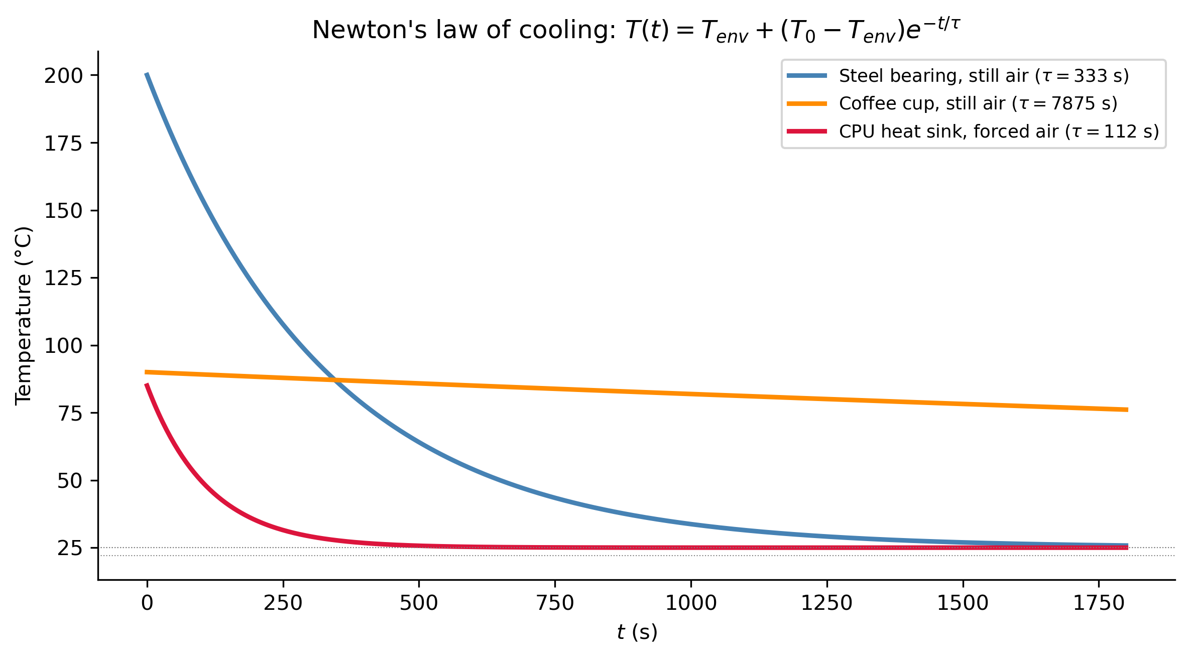
Figure 6: Combined convection–radiation cooling (COMB). Left: temperature history from a high-accuracy reference solution, showing the characteristic fast-then-slow cooling curve. Right: log–log convergence plot of the error in \(T\) at \(t=200\) s versus step size \(\Delta t\) for hand-coded Euler, Heun (improved Euler), and classical RK4. The measured slopes closely match the theoretical global orders \(O(\Delta t)\), \(O(\Delta t^2)\), and \(O(\Delta t^4)\) (dashed reference lines).
TipReading the Convergence Plot

On a log–log plot, a method with global error \(O(\Delta t^p)\) produces a straight line of slope \(p\). The measured Euler, Heun, and RK4 curves closely track the slope-1, slope-2, and slope-4 reference lines, respectively — a direct numerical confirmation of the orders of accuracy proved in Notes on numerical methods. Note also the practical payoff: to reach an error of about \(10^{-4}\) K at \(t=200\) s, Euler needs a step size around \(\Delta t \approx 0.002\) s (extrapolating the trend), while RK4 achieves it with \(\Delta t \approx 10\) s — several orders of magnitude fewer function evaluations for the same accuracy.


Part 7 (Enrichment) — The First Law and the Polytropic Piston–Cylinder

This bonus topic connects ODE modeling directly to thermodynamics in the sense mechanical engineers usually mean it — the first law applied to a compressible gas — and is a nice capstone for showing that Newton’s law of cooling, the ideal gas law, and the first law of thermodynamics all combine into a single first-order linear ODE.

Setup

Consider an ideal gas (mass \(m_g\), gas constant \(R\), constant-volume specific heat \(c_v\)) in a piston–cylinder assembly whose volume \(V(t)\) is prescribed externally (the piston moves at a controlled rate), while the gas simultaneously exchanges heat with the cylinder wall at temperature \(T_{env}\) via Newton’s law of cooling. The first law of thermodynamics for this closed system states: \[ dU = \delta Q - \delta W, \] where \(U = m_g c_v T\) is internal energy, \(\delta Q\) is heat added, and \(\delta W = P\,dV\) is work done by the gas as it expands. Using the ideal gas law \(P = m_gRT/V\) and Newton’s law for the heat exchange, \(\delta Q/dt = -hA(T-T_{env})\): \[ m_g c_v\,\frac{dT}{dt} = -hA(T-T_{env}) - \frac{m_gRT}{V(t)}\,\frac{dV}{dt}. \] Rearranging into standard linear-ODE form with \(V(t)\) prescribed (e.g. constant piston speed, \(V(t) = V_0 + vt\)): \[ \boxed{\frac{dT}{dt} + \left[\frac{hA}{m_gc_v} + \frac{R}{c_v}\frac{\dot V}{V(t)}\right]T = \frac{hA}{m_gc_v}T_{env}.} \tag{POLY} \] This is a first-order linear ODE with a time-varying coefficient — solvable in principle by the integrating factor method of Notes 2, though the integrating factor is most easily evaluated numerically here since \(V(t)\) is itself time-dependent.

ImportantRecovering the Adiabatic (Reversible) Limit

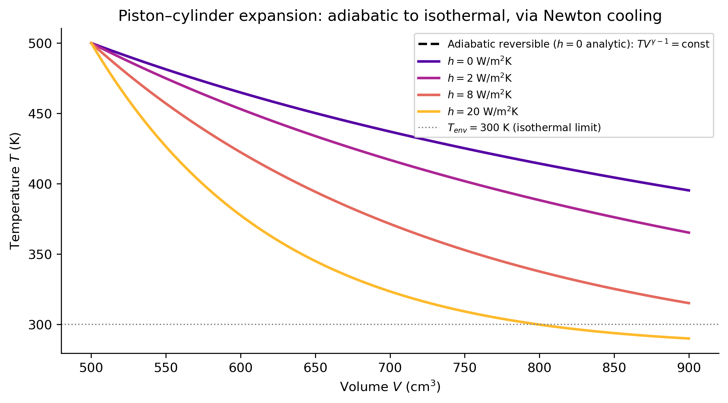
When \(h=0\) (a perfectly insulated cylinder — no heat exchange with the surroundings), (POLY) reduces to \(\dfrac{dT}{T} = -\dfrac{R}{c_v}\dfrac{dV}{V}\), which integrates directly to the familiar reversible adiabatic process relation from thermodynamics: \[ T V^{\gamma - 1} = \text{const}, \qquad \gamma = \frac{c_p}{c_v} = \frac{c_v+R}{c_v}. \] This is exactly the \(n=\gamma\) polytropic process from the course catalog description. With heat loss present (\(h>0\)), the gas cools faster than the adiabatic prediction — the process becomes an “effective” polytropic process with an exponent between the isothermal (\(n=1\)) and adiabatic (\(n=\gamma\)) limits, depending on how large \(h\) is relative to the piston speed.

Show the code
R_gas, cv_gas = 287.0, 718.0     # air, J/(kg K)
m_gas = 0.002                    # kg
A_wall = 0.01                    # m^2
Tenv_gas = 300.0                 # K
V0_gas, v_pist = 0.0005, 2.0e-5  # m^3, m^3/s
T0_gas = 500.0                   # K
t_end_gas = 20.0

def V_of_t(t): return V0_gas + v_pist*t

def make_rhs(h_val):
    def rhs(t, T):
        Vt = V_of_t(t)
        P = m_gas*R_gas*T/Vt
        dU_from_Q = -h_val*A_wall*(T-Tenv_gas)
        dW = P*v_pist
        return (dU_from_Q - dW)/(m_gas*cv_gas)
    return rhs

gamma_gas = (cv_gas+R_gas)/cv_gas
t_plot = np.linspace(0, t_end_gas, 400)
V_plot = V_of_t(t_plot)
T_adiabatic = T0_gas*(V0_gas/V_plot)**(gamma_gas-1)

fig, ax = plt.subplots(figsize=(8, 4.5))
ax.plot(V_plot*1e6, T_adiabatic, color='k', ls='--', lw=1.8, label=r'Adiabatic reversible ($h=0$ analytic): $TV^{\gamma-1}=$const')

for h_val, color in zip([0.0, 2.0, 8.0, 20.0], plt.cm.plasma(np.linspace(0.15, 0.85, 4))):
    sol = solve_ivp(make_rhs(h_val), (0, t_end_gas), [T0_gas], t_eval=t_plot, max_step=0.01)
    ax.plot(V_plot*1e6, sol.y[0], color=color, lw=2, label=f'$h={h_val:.0f}$ W/m$^2$K')

ax.axhline(Tenv_gas, color='gray', ls=':', lw=1, label='$T_{env}=300$ K (isothermal limit)')
ax.set_xlabel('Volume $V$ (cm$^3$)'); ax.set_ylabel('Temperature $T$ (K)')
ax.set_title('Piston–cylinder expansion: adiabatic to isothermal, via Newton cooling')
ax.legend(fontsize=8)
plt.tight_layout()
plt.show()

Figure 7: Piston–cylinder gas expansion with simultaneous heat loss to the cylinder wall. The gas expands at a fixed rate while losing heat according to Newton’s law with coefficient \(h\). As \(h\to 0\) the numerical solution converges exactly to the reversible adiabatic relation \(TV^{\gamma-1}=\text{const}\) (black dashed); increasing \(h\) pulls the process progressively toward the isothermal limit \(T=T_{env}\).

Connecting the Applications to the Course

Part 1: Cooling Part 3: Networks Part 4: Periodic forcing Part 5: Radiative Part 6: Combined Part 7 (bonus): Piston
ODE type 1st-order linear Linear system 1st-order linear, forced 1st-order nonlinear 1st-order, no closed form 1st-order linear, variable coeff.
Course topic First-order equations Linear systems Laplace transforms Nonlinear equations Numerical methods First-order equations
Key technique Separable / integrating factor Eigenvalues, eigenvectors Partial fractions in \(s\) Partial fractions in \(T\) Euler / Heun / RK4 Integrating factor (numeric)
Electrical analogue RC step response RC network RC filter frequency response — (no linear circuit analogue) Nonlinear circuit elements
TipLooking Ahead

Every application here reinforces that the type of ODE — not the physical subject it comes from — determines which solution technique applies. A mechanical engineering student who has seen Newton’s law of cooling will recognize the same integrating-factor technique the next time they meet a first-order linear ODE in an unrelated context (fluid draining, population growth, RC circuits); an electrical engineering student who has seen the thermal–electrical analogy will recognize that “solve the ODE” is a skill that transfers across their entire curriculum, not a fact specific to circuits. The nonlinear radiative law (Part 5) and the combined-mode problem (Part 6) also preview why numerical methods are indispensable in practice: most real engineering ODEs do not have closed-form solutions, and heat transfer is an excellent, physically motivated setting to introduce that fact.


References

Logan, J David. 2015. A First Course in Differential Equations, Third Edition.
Show the code
import sys
print("Python version:", sys.version)
print('\n'.join(f'{m.__name__}=={m.__version__}' for m in globals().values() if getattr(m, '__version__', None)))
Python version: 3.14.4 | packaged by conda-forge | (main, Apr  8 2026, 02:33:53) [Clang 20.1.8 ]
numpy==2.4.3
sympy==1.14.0
matplotlib==3.10.8

Reuse

CC BY-NC-SA 4.0