# This is a code cell that imports the necessary libraries for our session.import numpy as np # NumPy for numerical computationsimport scipy as sp # SciPy for scientific computingimport sympy as sym # SymPy for symbolic mathematicsimport matplotlib as mpl # Matplotlib for plottingimport matplotlib.pyplot as plt # Matplotlib pyplot interfacefrom scipy.integrate import solve_ivp # ODE solvermpl.rcParams['figure.dpi'] =150mpl.rcParams['axes.spines.top'] =Falsempl.rcParams['axes.spines.right'] =False
In this document, we will work through the details of showing that a particular function solves a particular differential equation. This is a common task in the study of differential equations, and it involves verifying that the function satisfies the equation when substituted into it.
Example 1
Here we will show both “by hand” and using SymPy that the function \(x(t) = \frac{1}{1+Ae^{-t}}\) is a solution to the ODE \(\frac{dx}{dt} = x(1-x)\).
By Hand
We want to verify that \[
x(t) = \frac{1}{1 + Ae^{-t}}
\] satisfies \(\dfrac{dx}{dt} = x(1-x)\) for every value of the constant \(A\).
Step 1 — Compute the left-hand side \(\dfrac{dx}{dt}\).
Since both sides are identical for every constant \(A\) and every \(t\), the function \(x(t) = \dfrac{1}{1+Ae^{-t}}\) is indeed a solution to \(\dfrac{dx}{dt} = x(1-x)\).
Note
Because \(A\) is an arbitrary constant, this is actually a one-parameter family of solutions — the general solution of this first-order ODE. A specific value of \(A\) is selected by imposing an initial condition.
Step 4 — Apply the initial condition \(x(0) = x_0\).
Setting \(t = 0\): \[
x(0) = \frac{1}{1 + A e^{0}} = \frac{1}{1+A} = x_0.
\] Solving for \(A\): \[
1 + A = \frac{1}{x_0} \quad \Longrightarrow \quad A = \frac{1}{x_0} - 1 = \frac{1-x_0}{x_0}.
\]
Substituting back and simplifying: \[
x(t) = \frac{1}{1 + \dfrac{1-x_0}{x_0}\,e^{-t}}
= \frac{x_0}{x_0 + (1-x_0)\,e^{-t}}.
\]
The solution to the initial value problem \[
\frac{dx}{dt} = x(1-x), \qquad x(0) = x_0
\] is therefore \[
\boxed{x(t) = \frac{x_0}{x_0 + (1-x_0)\,e^{-t}}}.
\]
Tip
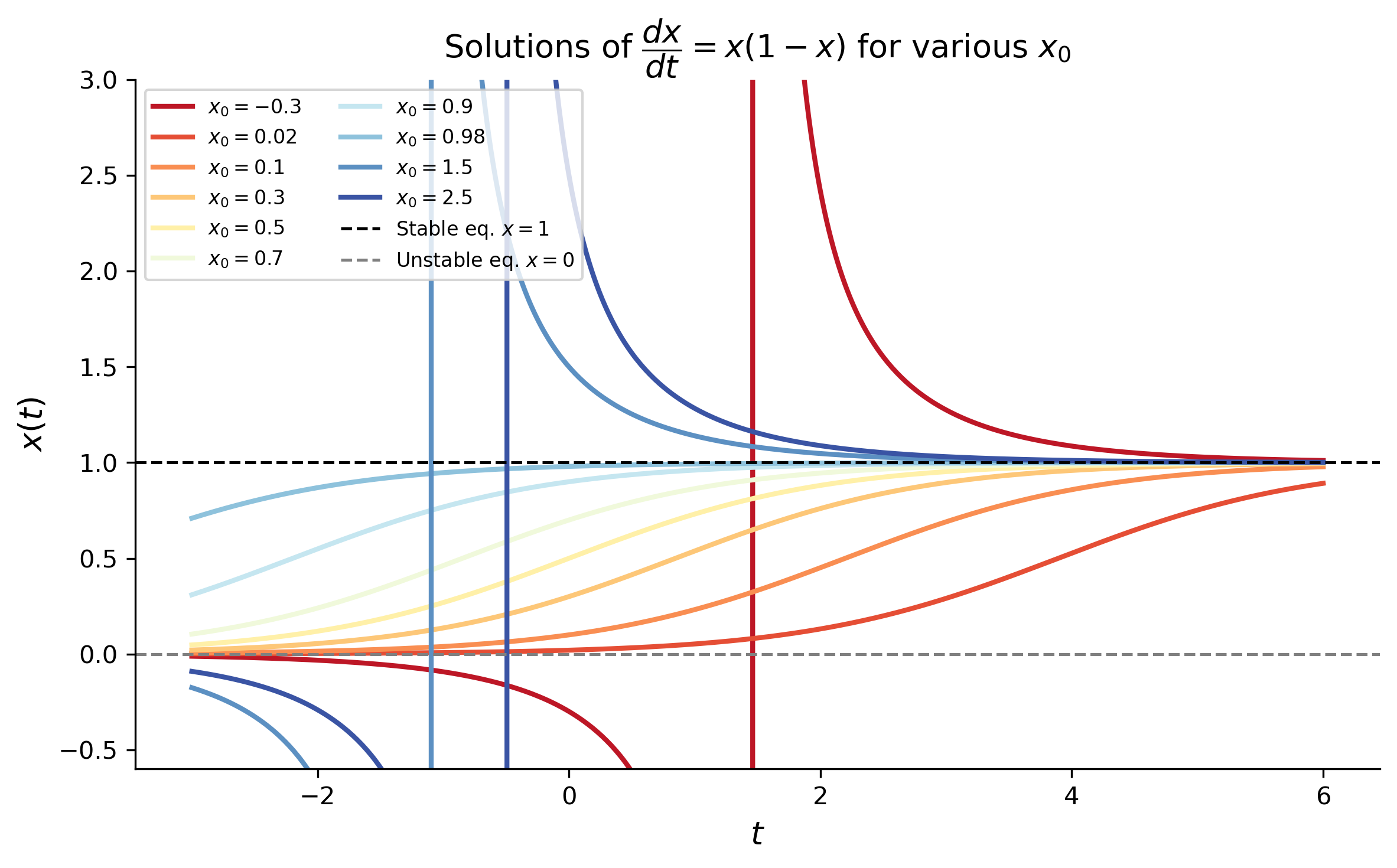
Long-run behavior. Since \(e^{-t} \to 0\) as \(t \to \infty\), we have \(x(t) \to 1\) for any \(x_0 \in (0, 1)\). The constant solution \(x = 1\) is a stable equilibrium. Likewise \(x = 0\) is an unstable equilibrium: solutions starting slightly above zero still move away toward \(x = 1\).
Using SymPy
We now confirm the above calculation symbolically using SymPy.
Define the symbols and the candidate solution.
t, A, x0 = sym.symbols('t A x_0', real=True)x = sym.S(1) / (1+ A * sym.exp(-t))from IPython.display import Math, displaydisplay(Math(r'x(t) = '+ sym.latex(x)))
\(\displaystyle x(t) = \frac{1}{A e^{- t} + 1}\)
Verify that \(\dfrac{dx}{dt} = x(1-x)\).
We compute both sides and subtract; if SymPy returns \(0\) the identity holds.
The plot below shows solution curves of the IVP \[
\frac{dx}{dt} = x(1-x), \qquad x(0) = x_0
\] for a range of initial values \(x_0\). The formula used is \(x(t) = \dfrac{x_0}{x_0 + (1-x_0)e^{-t}}\).
Figure 1: Solutions of \(dx/dt = x(1-x)\) for various initial conditions \(x_0\). All solutions with \(x_0 \in (0,1)\) increase toward the stable equilibrium \(x=1\) (upper dashed line), while solutions with \(x_0 > 1\) decrease toward it. The unstable equilibrium \(x=0\) (lower dashed line) repels nearby solutions.
References
TipExpand for Session Info
Show the code
import sys # sys for system-specific parameters and functionsprint("Python version:", sys.version)print('\n'.join(f'{m.__name__}=={m.__version__}'for m inglobals().values() ifgetattr(m, '__version__', None)))