Laplace Transforms — Definition and Basic Properties

Show the code
# This is a code cell that imports the necessary libraries for our session.
import sympy as sym                       # SymPy for symbolic mathematics
import numpy as np                        # NumPy for numerical computations
import matplotlib as mpl                  # Matplotlib for plotting
import matplotlib.pyplot as plt           # Matplotlib pyplot interface
from IPython.display import Math, display
mpl.rcParams['figure.dpi'] = 150
mpl.rcParams['axes.spines.top'] = False
mpl.rcParams['axes.spines.right'] = False

# Declare the symbolic variables used throughout
t, s = sym.symbols('t s', real=True)

In this document we work through fully solved examples for the topics covered in Section 3.1 of the text (Logan 2015): the definition of the Laplace transform, the basic operational properties (linearity, the shift property, the switching property), and techniques for finding inverse transforms (table look-up, partial fractions, and completing the square).


Reference: Key Laplace Transform Facts

The Laplace transform of \(f(t)\), defined for \(t \geq 0\), is \[ F(s) = \mathcal{L}[f(t)] = \int_0^{\infty} e^{-st} f(t)\,dt, \] whenever the integral converges.

Short Table

\(f(t)\) \(F(s) = \mathcal{L}[f(t)]\) Conditions
\(1\) \(\dfrac{1}{s}\) \(s > 0\)
\(t^n\) (\(n = 0,1,2,\ldots\)) \(\dfrac{n!}{s^{n+1}}\) \(s > 0\)
\(e^{at}\) \(\dfrac{1}{s-a}\) \(s > a\)
\(\sin(kt)\) \(\dfrac{k}{s^2+k^2}\) \(s > 0\)
\(\cos(kt)\) \(\dfrac{s}{s^2+k^2}\) \(s > 0\)
\(\sinh(kt)\) \(\dfrac{k}{s^2-k^2}\) \(s > |k|\)
\(\cosh(kt)\) \(\dfrac{s}{s^2-k^2}\) \(s > |k|\)
\(t^n e^{at}\) \(\dfrac{n!}{(s-a)^{n+1}}\) \(s > a\)
\(e^{at}\sin(kt)\) \(\dfrac{k}{(s-a)^2+k^2}\) \(s > a\)
\(e^{at}\cos(kt)\) \(\dfrac{s-a}{(s-a)^2+k^2}\) \(s > a\)
\(H(t-a)\,f(t-a)\) \(e^{-as}F(s)\) \(s > 0\)

Operational Properties

Linearity. \[ \mathcal{L}[\alpha f(t) + \beta g(t)] = \alpha F(s) + \beta G(s). \]

First Shift (Exponential Shift) Property. If \(\mathcal{L}[f(t)] = F(s)\), then \[ \mathcal{L}[e^{at}f(t)] = F(s - a). \]

Second Shift (Switching) Property. If \(\mathcal{L}[f(t)] = F(s)\), then \[ \mathcal{L}[H(t-a)\,f(t-a)] = e^{-as}F(s), \] or equivalently in inverse form, \[ \mathcal{L}^{-1}[e^{-as}F(s)] = H(t-a)\,f(t-a). \]


Part I — Forward Transforms

Example 1 — Linearity and the Table: \(2 - 3e^{4t} + t^2 e^{-t}\)

Find \(\mathcal{L}\!\left[2 - 3e^{4t} + t^2 e^{-t}\right]\).

By Hand

Apply linearity and match each term to a table entry.

Term 1: \(\mathcal{L}[2] = \dfrac{2}{s}.\)

Term 2: \(\mathcal{L}[-3e^{4t}] = -\dfrac{3}{s-4}.\)

Term 3: \(\mathcal{L}[t^2 e^{-t}]\). The table entry for \(t^n e^{at}\) with \(n = 2\) and \(a = -1\) gives \[ \mathcal{L}[t^2 e^{-t}] = \frac{2!}{(s-(-1))^{3}} = \frac{2}{(s+1)^3}. \]

Combining by linearity: \[ \boxed{\mathcal{L}\!\left[2 - 3e^{4t} + t^2 e^{-t}\right] = \frac{2}{s} - \frac{3}{s-4} + \frac{2}{(s+1)^3}.} \]

Using SymPy

f1 = 2 - 3*sym.exp(4*t) + t**2 * sym.exp(-t)
F1 = sym.laplace_transform(f1, t, s, noconds=True)
display(Math(
    r'\mathcal{L}\!\left[2 - 3e^{4t} + t^2 e^{-t}\right] = '
    + sym.latex(sym.simplify(F1))))

\(\displaystyle \mathcal{L}\!\left[2 - 3e^{4t} + t^2 e^{-t}\right] = \frac{2}{\left(s + 1\right)^{3}} - \frac{3}{s - 4} + \frac{2}{s}\)


Example 2 — Switching Property: \((t+1)H(t-2)\)

Find \(\mathcal{L}[(t+1)H(t-2)]\).

By Hand

The function \((t+1)H(t-2)\) switches on at \(t = 2\), but it is not yet in the standard switching form \(H(t-a)f(t-a)\) because the multiplying function is \(f(t) = t+1\), not \(f(t-2)\). We rewrite \(t+1\) in terms of \((t-2)\): \[ t + 1 = (t - 2) + 3. \] Therefore \[ (t+1)H(t-2) = (t-2)H(t-2) + 3H(t-2). \]

Each piece is now in standard switching form. Apply \(\mathcal{L}[H(t-a)f(t-a)] = e^{-as}F(s)\) with \(a = 2\):

  • \(\mathcal{L}[(t-2)H(t-2)]\): here \(f(t) = t\), so \(F(s) = 1/s^2\), giving \(e^{-2s}/s^2\).
  • \(\mathcal{L}[3H(t-2)]\): here \(f(t) = 3\), so \(F(s) = 3/s\), giving \(3e^{-2s}/s\).

Combining: \[ \boxed{\mathcal{L}[(t+1)H(t-2)] = \frac{e^{-2s}}{s^2} + \frac{3e^{-2s}}{s} = \frac{e^{-2s}(1 + 3s)}{s^2}.} \]

Tip

The rewriting trick. Whenever you see \(f(t)H(t-a)\) and \(f(t)\) is not naturally a function of \((t-a)\), write \(t = (t-a)+a\) (or expand \(f\) about \(t=a\)) to put the expression into standard switching form before applying the property.

Using SymPy

f2 = (t + 1)*sym.Heaviside(t - 2)
F2 = sym.laplace_transform(f2, t, s, noconds=True)
display(Math(
    r'\mathcal{L}[(t+1)H(t-2)] = '
    + sym.latex(sym.simplify(F2))))

\(\displaystyle \mathcal{L}[(t+1)H(t-2)] = \frac{\left(3 s + 1\right) e^{- 2 s}}{s^{2}}\)


Example 3 — Direct Table Look-up: \(\sin 3t\)

Find \(\mathcal{L}[\sin 3t]\).

By Hand

From the table with \(k = 3\): \[ \mathcal{L}[\sin(3t)] = \frac{3}{s^2 + 9}. \]

\[\boxed{\mathcal{L}[\sin 3t] = \frac{3}{s^2+9}.}\]

Using SymPy

F3 = sym.laplace_transform(sym.sin(3*t), t, s, noconds=True)
display(Math(r'\mathcal{L}[\sin 3t] = ' + sym.latex(F3)))

\(\displaystyle \mathcal{L}[\sin 3t] = \frac{3}{s^{2} + 9}\)


Example 4 — Angle Addition: \(\cos(t - \pi/2)\)

Find \(\mathcal{L}[\cos(t - \pi/2)]\).

By Hand

Expand using the angle subtraction formula \(\cos(\alpha - \beta) = \cos\alpha\cos\beta + \sin\alpha\sin\beta\): \[ \cos\!\left(t - \tfrac{\pi}{2}\right) = \cos t\cos\tfrac{\pi}{2} + \sin t\sin\tfrac{\pi}{2} = 0 + \sin t = \sin t. \]

Therefore: \[ \mathcal{L}\!\left[\cos\!\left(t - \tfrac{\pi}{2}\right)\right] = \mathcal{L}[\sin t] = \frac{1}{s^2+1}. \]

\[\boxed{\mathcal{L}\!\left[\cos\!\left(t - \tfrac{\pi}{2}\right)\right] = \frac{1}{s^2+1}.}\]

Note

This makes geometric sense: shifting \(\cos t\) to the right by \(\pi/2\) produces \(\sin t\). Compare the result with \(\mathcal{L}[\cos t] = s/(s^2+1)\) — the transforms are different because the functions differ for \(t > 0\).

Be careful: \(\cos(t - \pi/2)\) here is a simple trig identity, not a switched-on cosine. The switching property applies only when the Heaviside function \(H(t-a)\) is present.

Using SymPy

f4 = sym.cos(t - sym.pi/2)
F4 = sym.laplace_transform(f4, t, s, noconds=True)
display(Math(
    r'\mathcal{L}\!\left[\cos(t-\pi/2)\right] = '
    + sym.latex(sym.simplify(F4))))

\(\displaystyle \mathcal{L}\!\left[\cos(t-\pi/2)\right] = \frac{1}{s^{2} + 1}\)


Example 5 — First Shift Property with Hyperbolic Sine: \(5e^{2t}\sinh 3t\)

Find \(\mathcal{L}[5e^{2t}\sinh 3t]\).

By Hand

Use the first shift property: \(\mathcal{L}[e^{at}f(t)] = F(s-a)\).

Here \(a = 2\) and \(f(t) = 5\sinh 3t\).

From the table with \(k = 3\): \[ \mathcal{L}[\sinh 3t] = \frac{3}{s^2-9}, \qquad\text{so}\qquad \mathcal{L}[5\sinh 3t] = \frac{15}{s^2-9} =: F(s). \]

Replace \(s\) by \(s - 2\): \[ \mathcal{L}[5e^{2t}\sinh 3t] = F(s-2) = \frac{15}{(s-2)^2 - 9}. \]

Expand the denominator: \[ (s-2)^2 - 9 = s^2 - 4s + 4 - 9 = s^2 - 4s - 5 = (s-5)(s+1). \]

\[\boxed{\mathcal{L}[5e^{2t}\sinh 3t] = \frac{15}{(s-2)^2-9} = \frac{15}{(s-5)(s+1)}.}\]

Using SymPy

f5 = 5*sym.exp(2*t)*sym.sinh(3*t)
F5 = sym.laplace_transform(f5, t, s, noconds=True)
display(Math(
    r'\mathcal{L}[5e^{2t}\sinh 3t] = '
    + sym.latex(sym.simplify(F5))))

\(\displaystyle \mathcal{L}[5e^{2t}\sinh 3t] = \frac{15}{\left(s - 2\right)^{2} - 9}\)


Example 6 — Switching Property: \(H(t-2)\sin(t-2)\)

Find \(\mathcal{L}[H(t-2)\sin(t-2)]\).

By Hand

This is already in standard switching form \(H(t-a)f(t-a)\) with \(a = 2\) and \(f(t) = \sin t\).

From the table: \(F(s) = \mathcal{L}[\sin t] = \dfrac{1}{s^2+1}\).

By the switching property: \[ \mathcal{L}[H(t-2)\sin(t-2)] = e^{-2s}\cdot\frac{1}{s^2+1}. \]

\[\boxed{\mathcal{L}[H(t-2)\sin(t-2)] = \frac{e^{-2s}}{s^2+1}.}\]

Using SymPy

f6 = sym.Heaviside(t - 2)*sym.sin(t - 2)
F6 = sym.laplace_transform(f6, t, s, noconds=True)
display(Math(
    r'\mathcal{L}[H(t-2)\sin(t-2)] = '
    + sym.latex(sym.simplify(F6))))

\(\displaystyle \mathcal{L}[H(t-2)\sin(t-2)] = \frac{e^{- 2 s}}{s^{2} + 1}\)


Part II — Inverse Transforms

The principal techniques for finding inverse Laplace transforms are:

  1. Direct table look-up — recognise \(F(s)\) immediately.
  2. Linearity — split sums and pull out constants.
  3. Adjust the numerator — manufacture the table’s required numerator constant.
  4. Complete the square — handle shifted quadratic denominators.
  5. Partial fraction decomposition — break up rational functions.
  6. Switching property — handle factors of \(e^{-as}\).

Example 7 — Direct Table: \(\dfrac{4}{s-3}\)

Find \(\mathcal{L}^{-1}\!\left[\dfrac{4}{s-3}\right]\).

By Hand

Recognise \(\dfrac{1}{s-a}\) with \(a = 3\), scaled by \(4\): \[ \mathcal{L}^{-1}\!\left[\frac{4}{s-3}\right] = 4\,\mathcal{L}^{-1}\!\left[\frac{1}{s-3}\right] = 4e^{3t}. \]

\[\boxed{\mathcal{L}^{-1}\!\left[\frac{4}{s-3}\right] = 4e^{3t}.}\]

Using SymPy

F7 = sym.Integer(4)/(s - 3)
f7 = sym.inverse_laplace_transform(F7, s, t)
display(Math(
    r'\mathcal{L}^{-1}\!\left[\frac{4}{s-3}\right] = '
    + sym.latex(f7)))

\(\displaystyle \mathcal{L}^{-1}\!\left[\frac{4}{s-3}\right] = 4 e^{3 t} \theta\left(t\right)\)


Example 8 — Linearity and Adjusting the Numerator: \(\dfrac{5}{s} + \dfrac{3}{s^2+4}\)

Find \(\mathcal{L}^{-1}\!\left[\dfrac{5}{s} + \dfrac{3}{s^2+4}\right]\).

By Hand

Split using linearity.

Term 1: \(\mathcal{L}^{-1}\!\left[\dfrac{5}{s}\right] = 5\).

Term 2: \(\dfrac{3}{s^2+4}\). The table entry for \(\sin(kt)\) requires the form \(\dfrac{k}{s^2+k^2}\). Here \(k^2 = 4\) so \(k = 2\). The numerator needs to be \(2\), not \(3\), so we write: \[ \frac{3}{s^2+4} = \frac{3}{2}\cdot\frac{2}{s^2+4}. \]

Therefore \(\mathcal{L}^{-1}\!\left[\dfrac{3}{s^2+4}\right] = \dfrac{3}{2}\sin(2t)\).

Combining: \[ \boxed{\mathcal{L}^{-1}\!\left[\frac{5}{s} + \frac{3}{s^2+4}\right] = 5 + \frac{3}{2}\sin(2t).} \]

Tip

Adjusting the numerator. When the denominator is \(s^2 + k^2\) but the numerator is a constant \(c \neq k\), factor as \(\dfrac{c}{s^2+k^2} = \dfrac{c}{k}\cdot\dfrac{k}{s^2+k^2}\) and invert to get \(\dfrac{c}{k}\sin(kt)\).

Using SymPy

F8 = sym.Integer(5)/s + sym.Integer(3)/(s**2 + 4)
f8 = sym.inverse_laplace_transform(F8, s, t)
display(Math(
    r'\mathcal{L}^{-1}\!\left[\frac{5}{s}+\frac{3}{s^2+4}\right] = '
    + sym.latex(sym.simplify(f8))))

\(\displaystyle \mathcal{L}^{-1}\!\left[\frac{5}{s}+\frac{3}{s^2+4}\right] = \frac{\left(3 \sin{\left(2 t \right)} + 10\right) \theta\left(t\right)}{2}\)


Example 9 — Shifted Power: \(\dfrac{6}{(s+4)^3}\)

Find \(\mathcal{L}^{-1}\!\left[\dfrac{6}{(s+4)^3}\right]\).

By Hand

Recognise the shifted form \(\dfrac{n!}{(s-a)^{n+1}}\) with \(a = -4\) and \(n = 2\) (so \(n! = 2! = 2\) and \(n+1 = 3\)): \[ \frac{6}{(s+4)^3} = 3\cdot\frac{2!}{(s+4)^3}. \]

From the table, \(\mathcal{L}^{-1}\!\left[\dfrac{2!}{(s-(-4))^3}\right] = t^2 e^{-4t}\), so: \[ \mathcal{L}^{-1}\!\left[\frac{6}{(s+4)^3}\right] = 3t^2 e^{-4t}. \]

\[\boxed{\mathcal{L}^{-1}\!\left[\frac{6}{(s+4)^3}\right] = 3t^2 e^{-4t}.}\]

Using SymPy

F9 = sym.Integer(6)/(s + 4)**3
f9 = sym.inverse_laplace_transform(F9, s, t)
display(Math(
    r'\mathcal{L}^{-1}\!\left[\frac{6}{(s+4)^3}\right] = '
    + sym.latex(f9)))

\(\displaystyle \mathcal{L}^{-1}\!\left[\frac{6}{(s+4)^3}\right] = 3 t^{2} e^{- 4 t} \theta\left(t\right)\)


Example 10 — Switching Property: \(\dfrac{3}{s}e^{-2s}\)

Find \(\mathcal{L}^{-1}\!\left[\dfrac{3}{s}e^{-2s}\right]\).

By Hand

The factor \(e^{-2s}\) signals the switching property with \(a = 2\). The remaining factor \(F(s) = \dfrac{3}{s}\) inverts to \(f(t) = 3\).

By the switching property: \[ \mathcal{L}^{-1}\!\left[\frac{3}{s}e^{-2s}\right] = 3H(t-2). \]

\[\boxed{\mathcal{L}^{-1}\!\left[\frac{3}{s}e^{-2s}\right] = 3H(t-2).}\]

This represents a step function that jumps to the value \(3\) at \(t = 2\).

Using SymPy

F10 = (sym.Integer(3)/s)*sym.exp(-2*s)
f10 = sym.inverse_laplace_transform(F10, s, t)
display(Math(
    r'\mathcal{L}^{-1}\!\left[\frac{3}{s}e^{-2s}\right] = '
    + sym.latex(f10)))

\(\displaystyle \mathcal{L}^{-1}\!\left[\frac{3}{s}e^{-2s}\right] = 3 \theta\left(t - 2\right)\)


Example 11 — Partial Fractions with Switching: \(\dfrac{2}{s(s+4)}e^{-3s}\)

Find \(\mathcal{L}^{-1}\!\left[\dfrac{2}{s(s+4)}e^{-3s}\right]\).

By Hand

Step 1 — Identify \(a\) and \(F(s)\).

The factor \(e^{-3s}\) signals the switching property with \(a = 3\). We first find \(\mathcal{L}^{-1}\!\left[\dfrac{2}{s(s+4)}\right]\) and then shift.

Step 2 — Partial fraction decomposition of \(\dfrac{2}{s(s+4)}\).

\[ \frac{2}{s(s+4)} = \frac{A}{s} + \frac{B}{s+4}. \]

Multiply through by \(s(s+4)\): \[ 2 = A(s+4) + Bs. \]

Set \(s = 0\): \(2 = 4A \Rightarrow A = \dfrac{1}{2}\).

Set \(s = -4\): \(2 = -4B \Rightarrow B = -\dfrac{1}{2}\).

\[ \frac{2}{s(s+4)} = \frac{1/2}{s} - \frac{1/2}{s+4}. \]

Step 3 — Invert.

\[ \mathcal{L}^{-1}\!\left[\frac{2}{s(s+4)}\right] = \frac{1}{2} - \frac{1}{2}e^{-4t} =: f(t). \]

Step 4 — Apply the switching property with \(a = 3\).

\[ \mathcal{L}^{-1}\!\left[\frac{2}{s(s+4)}e^{-3s}\right] = H(t-3)\,f(t-3) = H(t-3)\cdot\frac{1}{2}\!\left(1 - e^{-4(t-3)}\right). \]

\[\boxed{\mathcal{L}^{-1}\!\left[\frac{2}{s(s+4)}e^{-3s}\right] = \frac{1}{2}H(t-3)\!\left(1 - e^{-4(t-3)}\right).}\]

Using SymPy

F11 = (sym.Integer(2)/(s*(s + 4)))*sym.exp(-3*s)
f11 = sym.inverse_laplace_transform(F11, s, t)
display(Math(
    r'\mathcal{L}^{-1}\!\left[\frac{2}{s(s+4)}e^{-3s}\right] = '
    + sym.latex(sym.simplify(f11))))

\(\displaystyle \mathcal{L}^{-1}\!\left[\frac{2}{s(s+4)}e^{-3s}\right] = \frac{\left(e^{4 t} - e^{12}\right) e^{- 4 t} \theta\left(t - 3\right)}{2}\)


Example 12 — Mixed Sinusoidal Numerator: \(\dfrac{4s - 3}{s^2 + 9}\)

Find \(\mathcal{L}^{-1}\!\left[\dfrac{4s-3}{s^2+9}\right]\).

By Hand

Split into a \(\cos\) part and a \(\sin\) part, matching the table forms \(\dfrac{s}{s^2+k^2}\) and \(\dfrac{k}{s^2+k^2}\) with \(k = 3\):

\[ \frac{4s-3}{s^2+9} = 4\cdot\frac{s}{s^2+9} - 3\cdot\frac{1}{s^2+9}. \]

For the second term, introduce the required factor of \(k = 3\): \[ 3\cdot\frac{1}{s^2+9} = 1\cdot\frac{3}{s^2+9}. \]

Therefore: \[ \mathcal{L}^{-1}\!\left[\frac{4s-3}{s^2+9}\right] = 4\cos(3t) - \sin(3t). \]

\[\boxed{\mathcal{L}^{-1}\!\left[\frac{4s-3}{s^2+9}\right] = 4\cos(3t) - \sin(3t).}\]

Using SymPy

F12 = (4*s - 3)/(s**2 + 9)
f12 = sym.inverse_laplace_transform(F12, s, t)
display(Math(
    r'\mathcal{L}^{-1}\!\left[\frac{4s-3}{s^2+9}\right] = '
    + sym.latex(sym.simplify(f12))))

\(\displaystyle \mathcal{L}^{-1}\!\left[\frac{4s-3}{s^2+9}\right] = \left(- \sin{\left(3 t \right)} + 4 \cos{\left(3 t \right)}\right) \theta\left(t\right)\)


Example 13 — Rescaling the Frequency: \(\dfrac{5}{3s^2 + 12}\)

Find \(\mathcal{L}^{-1}\!\left[\dfrac{5}{3s^2+12}\right]\).

By Hand

Factor out \(3\) from the denominator so it matches the table form \(s^2 + k^2\): \[ \frac{5}{3s^2+12} = \frac{5}{3}\cdot\frac{1}{s^2+4}. \]

Now \(k^2 = 4\) so \(k = 2\). Introduce the required numerator factor: \[ \frac{5}{3(s^2+4)} = \frac{5}{6}\cdot\frac{2}{s^2+4}. \]

Therefore: \[ \mathcal{L}^{-1}\!\left[\frac{5}{3s^2+12}\right] = \frac{5}{6}\sin(2t). \]

\[\boxed{\mathcal{L}^{-1}\!\left[\frac{5}{3s^2+12}\right] = \frac{5}{6}\sin(2t).}\]

Using SymPy

F13 = sym.Integer(5)/(3*s**2 + 12)
f13 = sym.inverse_laplace_transform(F13, s, t)
display(Math(
    r'\mathcal{L}^{-1}\!\left[\frac{5}{3s^2+12}\right] = '
    + sym.latex(sym.simplify(f13))))

\(\displaystyle \mathcal{L}^{-1}\!\left[\frac{5}{3s^2+12}\right] = \frac{5 \sin{\left(2 t \right)} \theta\left(t\right)}{6}\)


Example 14 — Switching with Sine: \(e^{-\pi s/2}\,\dfrac{4}{s^2+4}\)

Find \(\mathcal{L}^{-1}\!\left[e^{-\pi s/2}\,\dfrac{4}{s^2+4}\right]\).

By Hand

The factor \(e^{-\pi s/2}\) signals the switching property with \(a = \pi/2\). The remaining factor is \(F(s) = \dfrac{4}{s^2+4}\). With \(k = 2\): \[ F(s) = \frac{4}{s^2+4} = 2\cdot\frac{2}{s^2+4}, \] so \(f(t) = \mathcal{L}^{-1}[F(s)] = 2\sin(2t)\).

Applying the switching property: \[ \mathcal{L}^{-1}\!\left[e^{-\pi s/2}\frac{4}{s^2+4}\right] = H\!\left(t - \tfrac{\pi}{2}\right)\cdot 2\sin\!\left(2\!\left(t-\tfrac{\pi}{2}\right)\right). \]

We can simplify: \(2\sin(2t - \pi) = 2\sin(2t)\cos\pi = -2\sin(2t)\), so the expression can also be written as \(-2H(t-\pi/2)\sin(2t)\), though the shifted form makes the structure clearest.

\[\boxed{\mathcal{L}^{-1}\!\left[e^{-\pi s/2}\frac{4}{s^2+4}\right] = 2H\!\left(t-\tfrac{\pi}{2}\right)\sin\!\left(2t - \pi\right).}\]

Using SymPy

F14 = sym.exp(-sym.pi*s/2)*(sym.Integer(4)/(s**2 + 4))
f14 = sym.inverse_laplace_transform(F14, s, t)
display(Math(
    r'\mathcal{L}^{-1}\!\left[e^{-\pi s/2}\frac{4}{s^2+4}\right] = '
    + sym.latex(sym.simplify(f14))))

\(\displaystyle \mathcal{L}^{-1}\!\left[e^{-\pi s/2}\frac{4}{s^2+4}\right] = - 2 \sin{\left(2 t \right)} \theta\left(t - \frac{\pi}{2}\right)\)


Example 15 — Completing the Square: \(\dfrac{3s+7}{s^2+6s+13}\)

Find \(\mathcal{L}^{-1}\!\left[\dfrac{3s+7}{s^2+6s+13}\right]\).

By Hand

Step 1 — Complete the square in the denominator.

\[ s^2 + 6s + 13 = (s^2 + 6s + 9) + 4 = (s+3)^2 + 4. \]

So \(a = -3\) and \(k = 2\) in the shifted table entries.

Step 2 — Rewrite the numerator in terms of \((s+3)\).

\[ 3s + 7 = 3(s+3) - 9 + 7 = 3(s+3) - 2. \]

Step 3 — Split and match table forms.

\[ \frac{3s+7}{(s+3)^2+4} = \frac{3(s+3) - 2}{(s+3)^2+4} = 3\cdot\frac{s+3}{(s+3)^2+4} - 2\cdot\frac{1}{(s+3)^2+4}. \]

For the second term, introduce the factor \(k = 2\): \[ 2\cdot\frac{1}{(s+3)^2+4} = 1\cdot\frac{2}{(s+3)^2+4}. \]

Step 4 — Invert using \(a = -3\), \(k = 2\).

\[ \mathcal{L}^{-1}\!\left[\frac{s+3}{(s+3)^2+4}\right] = e^{-3t}\cos(2t), \qquad \mathcal{L}^{-1}\!\left[\frac{2}{(s+3)^2+4}\right] = e^{-3t}\sin(2t). \]

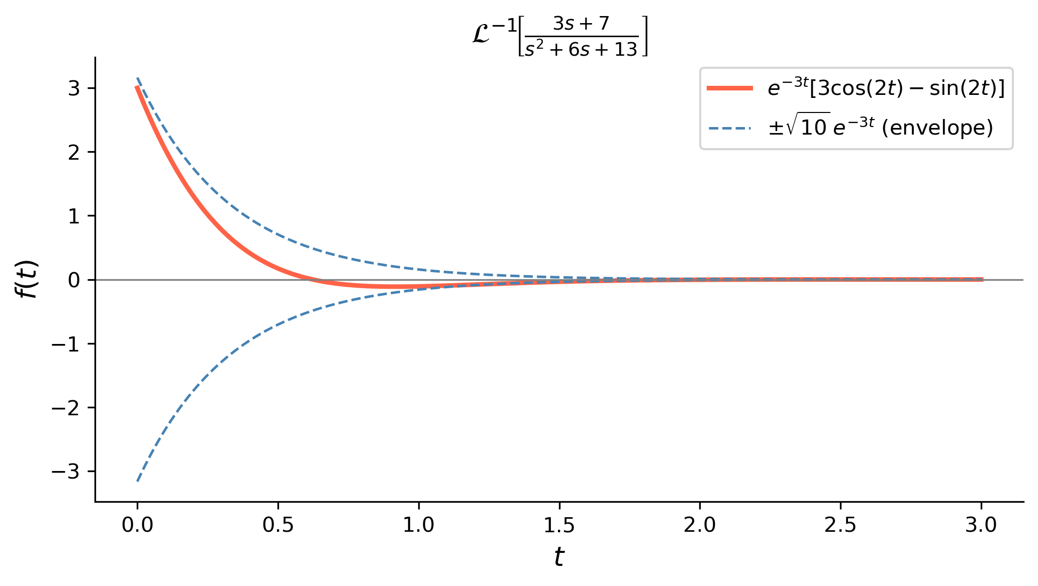
Therefore: \[ \mathcal{L}^{-1}\!\left[\frac{3s+7}{s^2+6s+13}\right] = 3e^{-3t}\cos(2t) - e^{-3t}\sin(2t). \]

\[\boxed{\mathcal{L}^{-1}\!\left[\frac{3s+7}{s^2+6s+13}\right] = e^{-3t}\!\left[3\cos(2t) - \sin(2t)\right].}\]

Using SymPy

F15 = (3*s + 7)/(s**2 + 6*s + 13)
f15 = sym.inverse_laplace_transform(F15, s, t)
display(Math(
    r'\mathcal{L}^{-1}\!\left[\frac{3s+7}{s^2+6s+13}\right] = '
    + sym.latex(sym.simplify(f15))))

\(\displaystyle \mathcal{L}^{-1}\!\left[\frac{3s+7}{s^2+6s+13}\right] = \left(- \sin{\left(2 t \right)} + 3 \cos{\left(2 t \right)}\right) e^{- 3 t} \theta\left(t\right)\)

Show the code
t_vals  = np.linspace(0, 3, 600)
f_vals  = np.exp(-3*t_vals)*(3*np.cos(2*t_vals) - np.sin(2*t_vals))
env_pos =  np.sqrt(10)*np.exp(-3*t_vals)   # amplitude = sqrt(3^2 + 1^2)
env_neg = -env_pos

fig, ax = plt.subplots(figsize=(7, 4))
ax.plot(t_vals, f_vals,  color='tomato',    lw=2.2,
        label=r'$e^{-3t}[3\cos(2t)-\sin(2t)]$')
ax.plot(t_vals, env_pos, color='steelblue', lw=1.2, ls='--',
        label=r'$\pm\sqrt{10}\,e^{-3t}$ (envelope)')
ax.plot(t_vals, env_neg, color='steelblue', lw=1.2, ls='--')
ax.axhline(0, color='gray', lw=0.8)
ax.set_xlabel(r'$t$', fontsize=13)
ax.set_ylabel(r'$f(t)$', fontsize=13)
ax.set_title(
    r'$\mathcal{L}^{-1}\!\left[\frac{3s+7}{s^2+6s+13}\right]$',
    fontsize=13)
ax.legend(fontsize=10)
plt.tight_layout()
plt.show()
Figure 1: The inverse transform \(f(t) = e^{-3t}[3\cos(2t)-\sin(2t)]\) from Example 15. The decaying exponential envelope \(\pm\sqrt{10}\,e^{-3t}\) is shown dashed.

Example 16 — Switching with a Delayed Ramp: \(\dfrac{5}{s^2}e^{-s}\)

Find \(\mathcal{L}^{-1}\!\left[\dfrac{5}{s^2}e^{-s}\right]\).

By Hand

The factor \(e^{-s}\) signals the switching property with \(a = 1\). The remaining factor \(F(s) = \dfrac{5}{s^2}\) inverts as: \[ \mathcal{L}^{-1}\!\left[\frac{5}{s^2}\right] = 5\,\mathcal{L}^{-1}\!\left[\frac{1!}{s^2}\right] = 5t =: f(t). \]

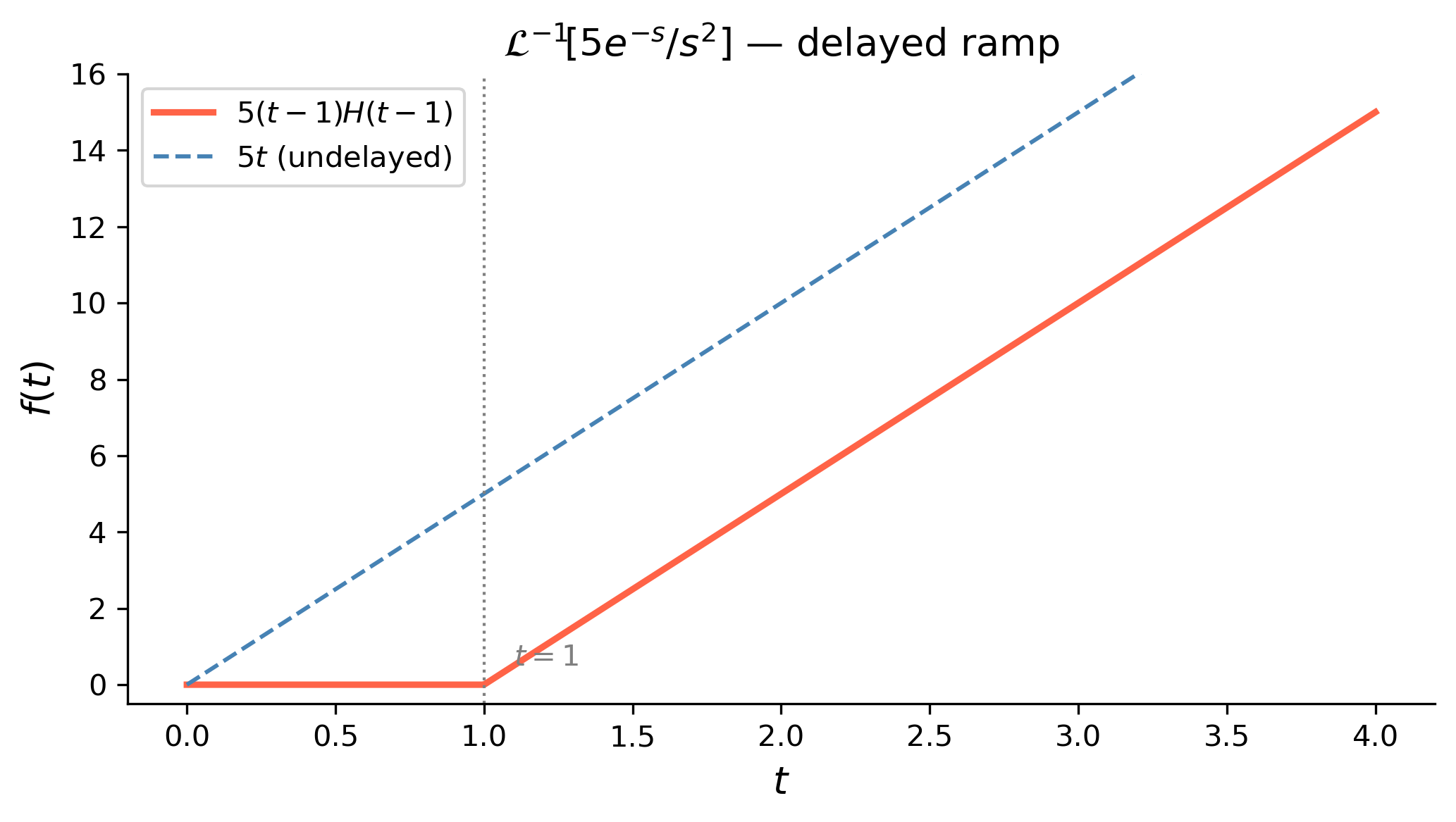
Applying the switching property: \[ \mathcal{L}^{-1}\!\left[\frac{5}{s^2}e^{-s}\right] = H(t-1)\,f(t-1) = 5(t-1)H(t-1). \]

\[\boxed{\mathcal{L}^{-1}\!\left[\frac{5}{s^2}e^{-s}\right] = 5(t-1)H(t-1).}\]

This is a delayed ramp: zero for \(t < 1\), then growing with slope \(5\) for \(t > 1\).

Using SymPy

F16 = (sym.Integer(5)/s**2)*sym.exp(-s)
f16 = sym.inverse_laplace_transform(F16, s, t)
display(Math(
    r'\mathcal{L}^{-1}\!\left[\frac{5}{s^2}e^{-s}\right] = '
    + sym.latex(sym.simplify(f16))))

\(\displaystyle \mathcal{L}^{-1}\!\left[\frac{5}{s^2}e^{-s}\right] = 5 \left(t - 1\right) \theta\left(t - 1\right)\)

Show the code
t_vals     = np.linspace(0, 4, 500)
f_delayed  = 5*(t_vals - 1)*np.where(t_vals >= 1, 1, 0)
f_undelayed = 5*t_vals

fig, ax = plt.subplots(figsize=(7, 4))
ax.plot(t_vals, f_delayed,   color='tomato',    lw=2.2,
        label=r'$5(t-1)H(t-1)$')
ax.plot(t_vals, f_undelayed, color='steelblue', lw=1.4, ls='--',
        label=r'$5t$ (undelayed)')
ax.axvline(1, color='gray', lw=1, ls=':')
ax.annotate(r'$t = 1$', xy=(1, 0.15), xytext=(1.1, 0.5),
            fontsize=10, color='gray')
ax.set_xlabel(r'$t$', fontsize=13)
ax.set_ylabel(r'$f(t)$', fontsize=13)
ax.set_title(
    r'$\mathcal{L}^{-1}\!\left[5e^{-s}/s^2\right]$ — delayed ramp',
    fontsize=13)
ax.legend(fontsize=10)
ax.set_ylim(-0.5, 16)
plt.tight_layout()
plt.show()
Figure 2: The delayed ramp \(5(t-1)H(t-1)\) from Example 16 (red) alongside the un-delayed ramp \(5t\) (dashed). The switch-on at \(t=1\) is clearly visible.

Work through these steps in order:

  1. Look for \(e^{-as}\). If present, factor it out, find \(\mathcal{L}^{-1}[F(s)]\) of the remaining piece, then apply the switching property: \(\mathcal{L}^{-1}[e^{-as}F(s)] = H(t-a)f(t-a)\).

  2. Check for a direct table match. \(\dfrac{c}{s-a}\), \(\dfrac{c}{s^2+k^2}\), \(\dfrac{cs}{s^2+k^2}\), \(\dfrac{c}{(s-a)^{n+1}}\) all have immediate inverses.

  3. Split mixed numerators. If the numerator is \(\alpha s + \beta\) over \(s^2 + k^2\) (or \((s-a)^2 + k^2\)), separate into \(\cos\)/\(\sin\) (or \(e^{at}\cos\)/\(e^{at}\sin\)) terms.

  4. Complete the square. If the denominator is a quadratic \(s^2 + bs + c\) with complex roots, write it as \((s-a)^2 + k^2\) and rewrite the numerator in terms of \((s-a)\) before inverting.

  5. Partial fractions. For a rational \(F(s)\) with real roots in the denominator, decompose into simpler fractions first, then invert each piece.


References

Logan, J David. 2015. A First Course in Differential Equations, Third Edition.
import sys
print("Python version:", sys.version)
print('\n'.join(f'{m.__name__}=={m.__version__}'
                for m in globals().values()
                if getattr(m, '__version__', None)))
Python version: 3.14.4 | packaged by conda-forge | (main, Apr  8 2026, 02:33:53) [Clang 20.1.8 ]
sympy==1.14.0
numpy==2.4.3
matplotlib==3.10.8

Reuse

CC BY-NC-SA 4.0