Solving Linear Systems — Worked Examples

# This is a code cell that imports the necessary libraries for our session.
import numpy as np                        # NumPy for numerical computations
import sympy as sym                       # SymPy for symbolic mathematics
import matplotlib as mpl                  # Matplotlib for plotting
import matplotlib.pyplot as plt           # Matplotlib pyplot interface
from IPython.display import Math, display
mpl.rcParams['figure.dpi'] = 150
mpl.rcParams['axes.spines.top'] = False
mpl.rcParams['axes.spines.right'] = False

In this document we work through fully solved examples for the topics covered in Section 4.4 of the text (Logan 2015):

• §4.4.1 — Solving \(2\times 2\) linear systems \(\mathbf{x}' = A\mathbf{x}\) when \(A\) has real, unequal eigenvalues: assembling the general solution from eigenpairs, classifying and sketching the phase portrait, and solving initial value problems.
• §4.4.2 — The case of complex conjugate eigenvalues \(\lambda = a \pm bi\): deriving real-valued solutions via Euler’s formula, phase portraits for spiral sinks/sources and stable centers, and IVPs.

Each example is worked “by hand” first and then verified using NumPy and/or SymPy.

---

§4.4.1 Real Unequal Eigenvalues

When the coefficient matrix \(A\) of the system \(\mathbf{x}' = A\mathbf{x}\) has two real, unequal eigenvalues \(\lambda_1 \neq \lambda_2\) with corresponding eigenvectors \(\mathbf{v}_1\) and \(\mathbf{v}_2\), a fundamental set of solutions is

\[ \mathbf{x}_1(t) = \mathbf{v}_1 e^{\lambda_1 t}, \qquad \mathbf{x}_2(t) = \mathbf{v}_2 e^{\lambda_2 t}, \]

and the general solution is

\[ \mathbf{x}(t) = c_1 \mathbf{v}_1 e^{\lambda_1 t} + c_2 \mathbf{v}_2 e^{\lambda_2 t}. \]

The type and stability of the equilibrium \(\mathbf{x}^* = \mathbf{0}\) are determined by the signs of \(\lambda_1\) and \(\lambda_2\):

Eigenvalue signs	Critical point type	Stability
\(\lambda_1 < \lambda_2 < 0\)	Stable node	Asymptotically stable
\(0 < \lambda_1 < \lambda_2\)	Unstable node	Unstable
\(\lambda_1 < 0 < \lambda_2\)	Saddle point	Unstable
\(\lambda_1 < 0 = \lambda_2\) or \(\lambda_1 = 0 < \lambda_2\)	Non-isolated equilibria	Not isolated

---

Example 1 — General Solution and Phase Portrait from Eigenpairs (Stable Node)

The matrix \(A\) of a linear system \(\mathbf{x}' = A\mathbf{x}\) has eigenpairs \[ \lambda_1 = -1,\; \mathbf{v}_1 = \begin{pmatrix} 1 \\ 3 \end{pmatrix}; \qquad \lambda_2 = -4,\; \mathbf{v}_2 = \begin{pmatrix} 2 \\ 1 \end{pmatrix}. \] Write the general solution, classify the critical point at the origin, and sketch the phase portrait.

By Hand

Step 1 — Assemble the fundamental solutions.

Each eigenpair \(\lambda_k, \mathbf{v}_k\) yields a solution \(\mathbf{x}_k(t) = \mathbf{v}_k e^{\lambda_k t}\):

\[ \mathbf{x}_1(t) = \begin{pmatrix} 1 \\ 3 \end{pmatrix} e^{-t}, \qquad \mathbf{x}_2(t) = \begin{pmatrix} 2 \\ 1 \end{pmatrix} e^{-4t}. \]

Step 2 — Write the general solution.

\[ \boxed{\mathbf{x}(t) = c_1 \begin{pmatrix} 1 \\ 3 \end{pmatrix} e^{-t} + c_2 \begin{pmatrix} 2 \\ 1 \end{pmatrix} e^{-4t}.} \]

In component form: \[ x(t) = c_1 e^{-t} + 2c_2 e^{-4t}, \qquad y(t) = 3c_1 e^{-t} + c_2 e^{-4t}. \]

Step 3 — Classify the critical point.

Both eigenvalues are negative: \(\lambda_1 = -1 < 0\) and \(\lambda_2 = -4 < 0\). As \(t \to +\infty\) both fundamental solutions decay to \(\mathbf{0}\), so every trajectory approaches the origin. The critical point is an asymptotically stable node (also called a sink).

Step 4 — Describe the phase portrait.

As \(t \to +\infty\) the faster-decaying term \(c_2 e^{-4t}\) becomes negligible relative to \(c_1 e^{-t}\), so all orbits (except those with \(c_1 = 0\)) become tangent to the eigenvector direction \(\mathbf{v}_1 = (1,3)^T\) near the origin. The two linear orbits — solutions with \(c_2 = 0\) or \(c_1 = 0\) — travel along the eigenvector directions toward the origin.

Tip

Dominant eigenvalue. When both eigenvalues are negative, the one closer to zero (here \(\lambda_1 = -1\)) is called the dominant eigenvalue because its corresponding term decays more slowly and governs the long-term direction of approach to the origin. The orbit tangent direction at the origin is therefore \(\mathbf{v}_1\).

Using NumPy and SymPy

t = sym.Symbol('t')
c1, c2 = sym.symbols('c1 c2')

lam1, lam2 = -1, -4
v1 = sym.Matrix([1, 3])
v2 = sym.Matrix([2, 1])

x_gen = c1 * v1 * sym.exp(lam1*t) + c2 * v2 * sym.exp(lam2*t)
display(Math(r'\mathbf{x}(t) = c_1 '
            + sym.latex(v1) + r'e^{-t} + c_2 '
            + sym.latex(v2) + r'e^{-4t}'))
display(Math(r'x(t) = ' + sym.latex(sym.simplify(x_gen[0]))))
display(Math(r'y(t) = ' + sym.latex(sym.simplify(x_gen[1]))))

\(\displaystyle \mathbf{x}(t) = c_1 \left[\begin{matrix}1\\3\end{matrix}\right]e^{-t} + c_2 \left[\begin{matrix}2\\1\end{matrix}\right]e^{-4t}\)

\(\displaystyle x(t) = c_{1} e^{- t} + 2 c_{2} e^{- 4 t}\)

\(\displaystyle y(t) = 3 c_{1} e^{- t} + c_{2} e^{- 4 t}\)

v1_np = np.array([1, 3], dtype=float)
v2_np = np.array([2, 1], dtype=float)

t_fwd = np.linspace(0,  5, 400)
t_bwd = np.linspace(0, -3, 400)

fig, ax = plt.subplots(figsize=(6, 6))
ax.axhline(0, color='gray', lw=0.7)
ax.axvline(0, color='gray', lw=0.7)

# Several orbits: vary (c1, c2)
for c1v, c2v in [(1, 0), (-1, 0), (0, 1), (0, -1),
                 (1,  1), (1, -1), (-1,  1), (-1, -1),
                 (2,  1), (-2, 1)]:
    for t_range in [t_fwd, t_bwd]:
        xc = c1v * v1_np[0] * np.exp(-1*t_range) + c2v * v2_np[0] * np.exp(-4*t_range)
        yc = c1v * v1_np[1] * np.exp(-1*t_range) + c2v * v2_np[1] * np.exp(-4*t_range)
        # Highlight pure eigenvector orbits
        if c2v == 0 and c1v != 0:
            ax.plot(xc, yc, color='tomato', lw=2.0, alpha=0.9)
        elif c1v == 0 and c2v != 0:
            ax.plot(xc, yc, color='steelblue', lw=2.0, alpha=0.9)
        else:
            ax.plot(xc, yc, color='gray', lw=1.0, alpha=0.5)

# Eigenvector direction arrows
ax.annotate('', xy=1.5*v1_np, xytext=np.zeros(2),
            arrowprops=dict(arrowstyle='->', color='tomato', lw=1.8))
ax.annotate('', xy=-1.5*v1_np, xytext=np.zeros(2),
            arrowprops=dict(arrowstyle='->', color='tomato', lw=1.8))
ax.annotate('', xy=1.5*v2_np, xytext=np.zeros(2),
            arrowprops=dict(arrowstyle='->', color='steelblue', lw=1.8))
ax.annotate('', xy=-1.5*v2_np, xytext=np.zeros(2),
            arrowprops=dict(arrowstyle='->', color='steelblue', lw=1.8))

ax.plot(0, 0, 'ko', ms=6, zorder=5)
ax.set_xlim(-4, 4)
ax.set_ylim(-5, 5)
ax.set_aspect('equal')
ax.set_xlabel(r'$x$', fontsize=13)
ax.set_ylabel(r'$y$', fontsize=13)
ax.set_title('Asymptotically stable node: '
             r'$\lambda_1=-1,\;\lambda_2=-4$', fontsize=11)
from matplotlib.lines import Line2D
legend_handles = [
    Line2D([0],[0], color='tomato',    lw=2, label=r'Linear orbit along $\mathbf{v}_1$'),
    Line2D([0],[0], color='steelblue', lw=2, label=r'Linear orbit along $\mathbf{v}_2$'),
    Line2D([0],[0], color='gray',      lw=1, label='Other orbits'),
]
ax.legend(handles=legend_handles, fontsize=9, loc='upper right')
plt.tight_layout()
plt.show()

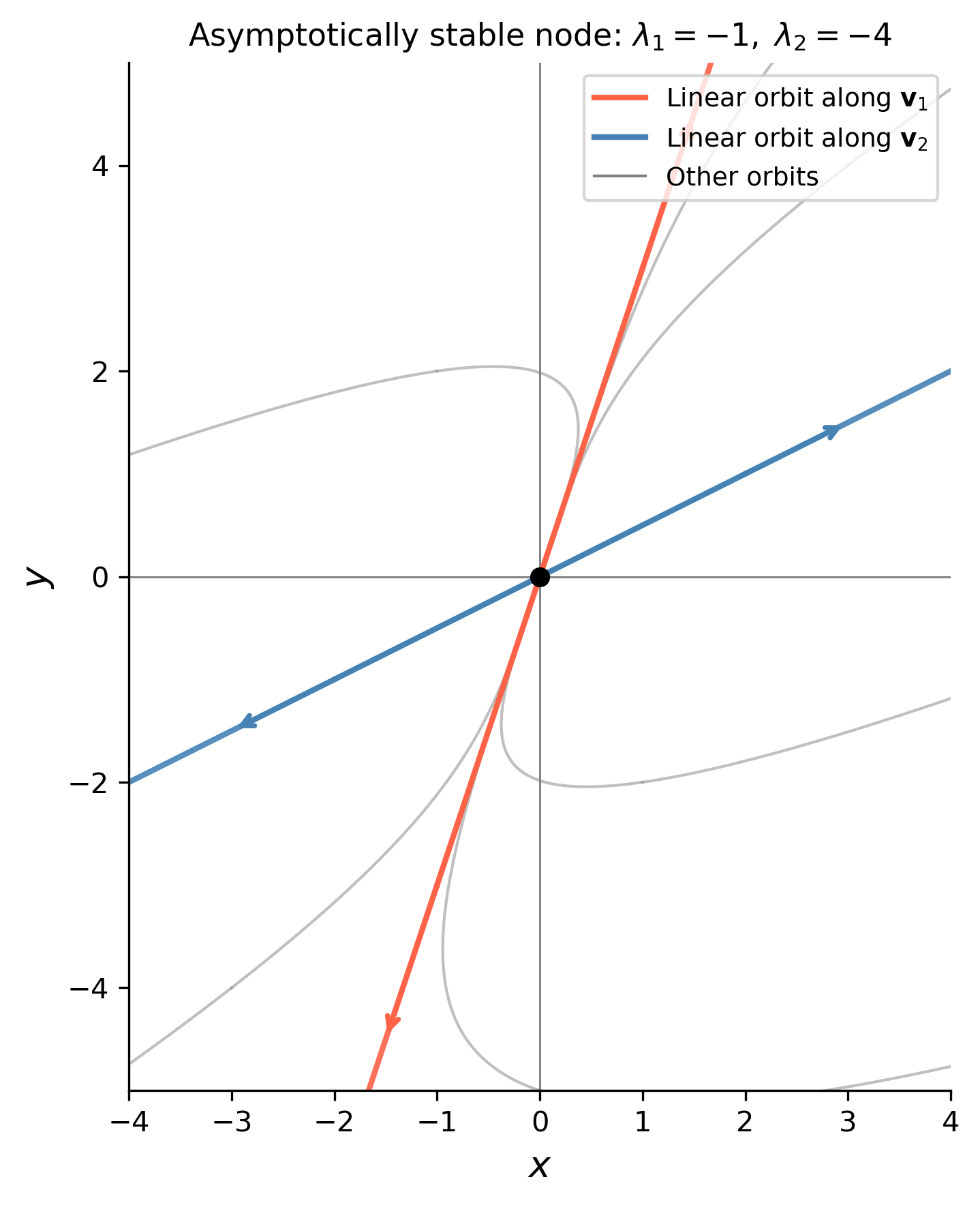
Figure 1: Phase portrait for Example 1: asymptotically stable node with eigenvalues \(\lambda_1=-1\) and \(\lambda_2=-4\). The linear orbits along \(\mathbf{v}_1=(1,3)^T\) (tomato) and \(\mathbf{v}_2=(2,1)^T\) (steelblue) are highlighted; all other orbits approach the origin tangent to \(\mathbf{v}_1\).

---

Example 2 — Full Solution from the Coefficient Matrix (Saddle Point)

Find the general solution of the system \[ \mathbf{x}' = A\mathbf{x}, \qquad A = \begin{pmatrix} 2 & 3 \\ 1 & 4 \end{pmatrix}, \] classify the critical point at the origin, and sketch the phase portrait.

By Hand

Step 1 — Characteristic equation.

\[ \det(A - \lambda I) = \det\begin{pmatrix} 2-\lambda & 3 \\ 1 & 4-\lambda \end{pmatrix} = (2-\lambda)(4-\lambda) - 3 = \lambda^2 - 6\lambda + 5 = (\lambda - 1)(\lambda - 5) = 0. \]

\[ \lambda_1 = 1, \qquad \lambda_2 = 5. \]

Since \(0 < \lambda_1 < \lambda_2\), the origin is an unstable node.

Note

Quick check. \(\text{tr}(A) = 2 + 4 = 6 = \lambda_1 + \lambda_2\) \(\checkmark\) and \(\det(A) = 8 - 3 = 5 = \lambda_1 \lambda_2\) \(\checkmark\).

Step 2 — Eigenvector for \(\lambda_1 = 1\).

Solve \((A - I)\mathbf{v} = \mathbf{0}\):

\[ \begin{pmatrix} 1 & 3 \\ 1 & 3 \end{pmatrix} \begin{pmatrix} v_1 \\ v_2 \end{pmatrix} = \mathbf{0} \quad\Longrightarrow\quad v_1 + 3v_2 = 0 \quad\Longrightarrow\quad v_1 = -3v_2. \]

Take \(v_2 = 1\): \(\quad \mathbf{v}_1 = \begin{pmatrix} -3 \\ 1 \end{pmatrix}\).

Step 3 — Eigenvector for \(\lambda_2 = 5\).

Solve \((A - 5I)\mathbf{v} = \mathbf{0}\):

\[ \begin{pmatrix} -3 & 3 \\ 1 & -1 \end{pmatrix} \begin{pmatrix} v_1 \\ v_2 \end{pmatrix} = \mathbf{0} \quad\Longrightarrow\quad v_1 = v_2. \]

Take \(v_2 = 1\): \(\quad \mathbf{v}_2 = \begin{pmatrix} 1 \\ 1 \end{pmatrix}\).

Step 4 — General solution.

\[ \boxed{\mathbf{x}(t) = c_1 \begin{pmatrix} -3 \\ 1 \end{pmatrix} e^{t} + c_2 \begin{pmatrix} 1 \\ 1 \end{pmatrix} e^{5t}.} \]

In component form: \[ x(t) = -3c_1 e^{t} + c_2 e^{5t}, \qquad y(t) = c_1 e^{t} + c_2 e^{5t}. \]

Both eigenvalues are positive, so every orbit (except the equilibrium itself) moves away from the origin as \(t \to +\infty\). The origin is an unstable node (also called a source).

Using SymPy

A2 = sym.Matrix([[2, 3], [1, 4]])
lam = sym.Symbol('lambda')

char2 = A2.charpoly(lam)
display(Math(r'\text{Characteristic polynomial: }\quad'
            + sym.latex(sym.Eq(char2.as_expr(), 0))))

for ev, mult, evecs in A2.eigenvects():
    display(Math(r'\lambda = ' + sym.latex(ev)
                 + r',\quad \mathbf{v} = ' + sym.latex(evecs[0])))

c1, c2 = sym.symbols('c1 c2')
ev_list = [(ev, evecs[0]) for ev, mult, evecs in A2.eigenvects()]
ev_list.sort(key=lambda p: float(p[0]))
x_gen2 = c1*ev_list[0][1]*sym.exp(ev_list[0][0]*t) \
        + c2*ev_list[1][1]*sym.exp(ev_list[1][0]*t)
display(Math(r'x(t) = ' + sym.latex(sym.simplify(x_gen2[0]))))
display(Math(r'y(t) = ' + sym.latex(sym.simplify(x_gen2[1]))))

\(\displaystyle \text{Characteristic polynomial: }\quad\lambda^{2} - 6 \lambda + 5 = 0\)

\(\displaystyle \lambda = 1,\quad \mathbf{v} = \left[\begin{matrix}-3\\1\end{matrix}\right]\)

\(\displaystyle \lambda = 5,\quad \mathbf{v} = \left[\begin{matrix}1\\1\end{matrix}\right]\)

\(\displaystyle x(t) = \left(- 3 c_{1} + c_{2} e^{4 t}\right) e^{t}\)

\(\displaystyle y(t) = \left(c_{1} + c_{2} e^{4 t}\right) e^{t}\)

v1_np = np.array([-3, 1], dtype=float)
v2_np = np.array([1,  1], dtype=float)

t_fwd = np.linspace(0,  1.0, 400)
t_bwd = np.linspace(0, -3.0, 400)

fig, ax = plt.subplots(figsize=(6, 6))
ax.axhline(0, color='gray', lw=0.7)
ax.axvline(0, color='gray', lw=0.7)

for c1v, c2v in [(1, 0), (-1, 0), (0, 1), (0, -1),
                 (1, 0.3), (-1, 0.3), (1, -0.3), (-1, -0.3),
                 (0.5, 0.5), (-0.5, -0.5)]:
    for t_range in [t_fwd, t_bwd]:
        xc = c1v*v1_np[0]*np.exp(1*t_range) + c2v*v2_np[0]*np.exp(5*t_range)
        yc = c1v*v1_np[1]*np.exp(1*t_range) + c2v*v2_np[1]*np.exp(5*t_range)
        mask = (np.abs(xc) < 5) & (np.abs(yc) < 5)
        if c2v == 0 and c1v != 0:
            ax.plot(xc[mask], yc[mask], color='tomato', lw=2.0, alpha=0.9)
        elif c1v == 0 and c2v != 0:
            ax.plot(xc[mask], yc[mask], color='steelblue', lw=2.0, alpha=0.9)
        else:
            ax.plot(xc[mask], yc[mask], color='gray', lw=1.0, alpha=0.5)

ax.plot(0, 0, 'ko', ms=6, zorder=5)
ax.set_xlim(-5, 5)
ax.set_ylim(-5, 5)
ax.set_aspect('equal')
ax.set_xlabel(r'$x$', fontsize=13)
ax.set_ylabel(r'$y$', fontsize=13)
ax.set_title(r'Unstable node: $\lambda_1=1,\;\lambda_2=5$', fontsize=11)
from matplotlib.lines import Line2D
legend_handles = [
    Line2D([0],[0], color='tomato',    lw=2, label=r'Linear orbit along $\mathbf{v}_1$'),
    Line2D([0],[0], color='steelblue', lw=2, label=r'Linear orbit along $\mathbf{v}_2$'),
    Line2D([0],[0], color='gray',      lw=1, label='Other orbits'),
]
ax.legend(handles=legend_handles, fontsize=9, loc='upper right')
plt.tight_layout()
plt.show()

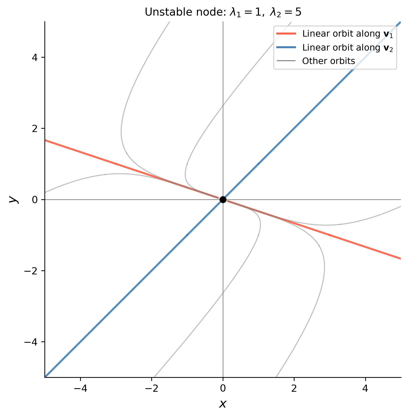
Figure 2: Phase portrait for Example 2: unstable node with \(\lambda_1=1\) and \(\lambda_2=5\). Orbits along the eigenvector directions are highlighted; all trajectories move away from the origin.

---

Example 3 — Initial Value Problem (Saddle Point)

Solve the initial value problem \[ \mathbf{x}' = \begin{pmatrix} -1 & 4 \\ 1 & -4 \end{pmatrix}\mathbf{x}, \qquad \mathbf{x}(0) = \begin{pmatrix} 2 \\ 1 \end{pmatrix}. \]

By Hand

Step 1 — Characteristic equation.

\[ \det(A - \lambda I) = \det\begin{pmatrix} -1-\lambda & 4 \\ 1 & -4-\lambda \end{pmatrix} = (-1-\lambda)(-4-\lambda) - 4 = \lambda^2 + 5\lambda + 4 - 4 = \lambda^2 + 5\lambda = \lambda(\lambda + 5). \]

\[ \lambda_1 = 0, \qquad \lambda_2 = -5. \]

Note

Zero eigenvalue. \(\det A = (−1)(−4) − (4)(1) = 0\), which confirms \(\lambda = 0\) is an eigenvalue. A zero eigenvalue always occurs when \(\det A = 0\) and signals a line of non-isolated equilibria in the direction of the corresponding eigenvector.

Step 2 — Eigenvector for \(\lambda_1 = 0\).

Solve \(A\mathbf{v} = \mathbf{0}\):

\[ \begin{pmatrix} -1 & 4 \\ 1 & -4 \end{pmatrix} \begin{pmatrix} v_1 \\ v_2 \end{pmatrix} = \mathbf{0} \quad\Longrightarrow\quad -v_1 + 4v_2 = 0 \quad\Longrightarrow\quad v_1 = 4v_2. \]

Take \(v_2 = 1\): \(\quad \mathbf{v}_1 = \begin{pmatrix} 4 \\ 1 \end{pmatrix}\).

Step 3 — Eigenvector for \(\lambda_2 = -5\).

Solve \((A + 5I)\mathbf{v} = \mathbf{0}\):

\[ \begin{pmatrix} 4 & 4 \\ 1 & 1 \end{pmatrix} \begin{pmatrix} v_1 \\ v_2 \end{pmatrix} = \mathbf{0} \quad\Longrightarrow\quad v_1 + v_2 = 0 \quad\Longrightarrow\quad v_1 = -v_2. \]

Take \(v_2 = 1\): \(\quad \mathbf{v}_2 = \begin{pmatrix} -1 \\ 1 \end{pmatrix}\).

Step 4 — General solution.

\[ \mathbf{x}(t) = c_1 \begin{pmatrix} 4 \\ 1 \end{pmatrix} + c_2 \begin{pmatrix} -1 \\ 1 \end{pmatrix} e^{-5t}. \]

Step 5 — Apply the initial condition \(\mathbf{x}(0) = (2,1)^T\).

At \(t = 0\):

\[ \begin{pmatrix} 4 & -1 \\ 1 & 1 \end{pmatrix} \begin{pmatrix} c_1 \\ c_2 \end{pmatrix} = \begin{pmatrix} 2 \\ 1 \end{pmatrix}. \]

The determinant of the coefficient matrix is \(4(1) - (-1)(1) = 5 \neq 0\). Using Cramer’s rule:

\[ c_1 = \frac{\det\begin{pmatrix} 2 & -1 \\ 1 & 1 \end{pmatrix}}{5} = \frac{2+1}{5} = \frac{3}{5}, \qquad c_2 = \frac{\det\begin{pmatrix} 4 & 2 \\ 1 & 1 \end{pmatrix}}{5} = \frac{4-2}{5} = \frac{2}{5}. \]

Step 6 — Particular solution.

\[ \boxed{\mathbf{x}(t) = \frac{3}{5}\begin{pmatrix} 4 \\ 1 \end{pmatrix} + \frac{2}{5}\begin{pmatrix} -1 \\ 1 \end{pmatrix} e^{-5t},} \]

or in component form:

\[ x(t) = \frac{12}{5} - \frac{2}{5}e^{-5t}, \qquad y(t) = \frac{3}{5} + \frac{2}{5}e^{-5t}. \]

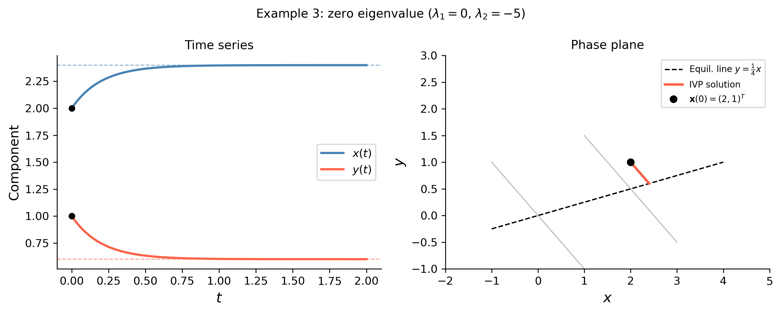
As \(t \to +\infty\), \(\mathbf{x}(t) \to c_1 \mathbf{v}_1 = \tfrac{3}{5}(4,1)^T\), a non-isolated equilibrium on the line \(y = \tfrac{1}{4}x\).

Using SymPy

A3 = sym.Matrix([[-1, 4], [1, -4]])
x0 = sym.Matrix([2, 1])

# General solution via dsolve
x_vec = sym.Matrix([sym.Function('x')(t), sym.Function('y')(t)])
ode_sys = x_vec.diff(t) - A3*x_vec

sol = sym.dsolve([sym.Eq(x_vec[0].diff(t), (A3*x_vec)[0]),
                  sym.Eq(x_vec[1].diff(t), (A3*x_vec)[1])])
for eq in sol:
    display(Math(sym.latex(eq)))

# Solve IVP
ics = {x_vec[0].subs(t,0): x0[0], x_vec[1].subs(t,0): x0[1]}
sol_ivp = sym.dsolve([sym.Eq(x_vec[0].diff(t), (A3*x_vec)[0]),
                      sym.Eq(x_vec[1].diff(t), (A3*x_vec)[1])], ics=ics)
display(Math(r'\text{IVP solution:}'))
for eq in sol_ivp:
    display(Math(sym.latex(eq)))

\(\displaystyle x{\left(t \right)} = 4 C_{1} - C_{2} e^{- 5 t}\)

\(\displaystyle y{\left(t \right)} = C_{1} + C_{2} e^{- 5 t}\)

\(\displaystyle \text{IVP solution:}\)

\(\displaystyle x{\left(t \right)} = \frac{12}{5} - \frac{2 e^{- 5 t}}{5}\)

\(\displaystyle y{\left(t \right)} = \frac{3}{5} + \frac{2 e^{- 5 t}}{5}\)

t_vals = np.linspace(0, 2, 500)

x_sol = 12/5 - (2/5)*np.exp(-5*t_vals)
y_sol =  3/5 + (2/5)*np.exp(-5*t_vals)

fig, axes = plt.subplots(1, 2, figsize=(10, 4))

# Left: time series
ax = axes[0]
ax.plot(t_vals, x_sol, color='steelblue', lw=2, label=r'$x(t)$')
ax.plot(t_vals, y_sol, color='tomato',    lw=2, label=r'$y(t)$')
ax.axhline(12/5, color='steelblue', lw=0.9, ls='--', alpha=0.6)
ax.axhline( 3/5, color='tomato',    lw=0.9, ls='--', alpha=0.6)
ax.plot(0, 2, 'ko', ms=5)
ax.plot(0, 1, 'ko', ms=5)
ax.set_xlabel(r'$t$', fontsize=13)
ax.set_ylabel('Component', fontsize=12)
ax.set_title('Time series', fontsize=11)
ax.legend(fontsize=10)

# Right: phase plane
ax = axes[1]
# Line of equilibria: y = x/4
x_line = np.linspace(-1, 4, 200)
ax.plot(x_line, x_line/4, 'k--', lw=1.2, label=r'Equil. line $y=\frac{1}{4}x$')

# Several orbits
v1_np = np.array([4, 1], dtype=float)
v2_np = np.array([-1, 1], dtype=float)
for c1v, c2v in [(3/5, 2/5), (1, 0), (-1, 0), (0, 1), (0, -1),
                 (0.5, 1), (0.5, -1), (-0.5, 1)]:
    xc = c1v*v1_np[0] + c2v*v2_np[0]*np.exp(-5*t_vals)
    yc = c1v*v1_np[1] + c2v*v2_np[1]*np.exp(-5*t_vals)
    if c1v == 3/5 and c2v == 2/5:
        ax.plot(xc, yc, color='tomato', lw=2.2, zorder=4,
                label='IVP solution')
    else:
        ax.plot(xc, yc, color='gray', lw=1.0, alpha=0.5)

ax.plot(2, 1, 'ko', ms=6, zorder=5, label=r'$\mathbf{x}(0)=(2,1)^T$')
ax.set_xlim(-2, 5)
ax.set_ylim(-1, 3)
ax.set_xlabel(r'$x$', fontsize=13)
ax.set_ylabel(r'$y$', fontsize=13)
ax.set_title('Phase plane', fontsize=11)
ax.legend(fontsize=8)

plt.suptitle(r"Example 3: zero eigenvalue ($\lambda_1=0$, $\lambda_2=-5$)",
             fontsize=11)
plt.tight_layout()
plt.show()

Figure 3: Solution of the IVP in Example 3. The particular solution (tomato) starts at \((2,1)\) and converges to \(\frac{3}{5}(4,1)^T \approx (2.4, 0.6)\) on the line of equilibria \(y = \frac{1}{4}x\) (dashed).

---

§4.4.2 Complex Eigenvalues

When \(A\) has complex conjugate eigenvalues \(\lambda = a \pm bi\) (with \(b \neq 0\)), the corresponding eigenvectors are also complex conjugates, \(\mathbf{v} = \mathbf{w} \pm i\mathbf{z}\). Taking one eigenpair \(a+bi,\; \mathbf{w}+i\mathbf{z}\) and applying Euler’s formula to expand \(({\mathbf{w}+i\mathbf{z}})e^{(a+bi)t}\) yields two real independent solutions:

\[ \mathbf{x}_1(t) = e^{at}(\mathbf{w}\cos bt - \mathbf{z}\sin bt), \qquad \mathbf{x}_2(t) = e^{at}(\mathbf{w}\sin bt + \mathbf{z}\cos bt), \]

and the general solution is

\[ \mathbf{x}(t) = c_1 e^{at}(\mathbf{w}\cos bt - \mathbf{z}\sin bt) + c_2 e^{at}(\mathbf{w}\sin bt + \mathbf{z}\cos bt). \]

The stability of the origin depends on the sign of \(a = \operatorname{Re}(\lambda)\):

Sign of \(a\)	Phase portrait	Stability
\(a < 0\)	Spiral sink	Asymptotically stable
\(a = 0\)	Center (closed ellipses)	Stable
\(a > 0\)	Spiral source	Unstable

---

Example 4 — Complex Eigenvalues: Spiral Sink

Find the general solution of the system \[ \mathbf{x}' = \begin{pmatrix} -1 & -3 \\ 3 & -1 \end{pmatrix}\mathbf{x}, \] and sketch the phase portrait.

By Hand

Step 1 — Characteristic equation.

\[ \det(A - \lambda I) = \det\begin{pmatrix} -1-\lambda & -3 \\ 3 & -1-\lambda \end{pmatrix} = (-1-\lambda)^2 + 9 = \lambda^2 + 2\lambda + 10 = 0. \]

Step 2 — Eigenvalues.

\[ \lambda = \frac{-2 \pm \sqrt{4 - 40}}{2} = \frac{-2 \pm 6i}{2} = -1 \pm 3i. \]

So \(a = -1\) and \(b = 3\).

Step 3 — Eigenvector for \(\lambda = -1 + 3i\).

Solve \((A - \lambda I)\mathbf{v} = \mathbf{0}\):

\[ \begin{pmatrix} -1-(-1+3i) & -3 \\ 3 & -1-(-1+3i) \end{pmatrix} = \begin{pmatrix} -3i & -3 \\ 3 & -3i \end{pmatrix}. \]

Using the first row: \(-3iv_1 - 3v_2 = 0 \Rightarrow v_2 = -iv_1\). Choose \(v_1 = 1\), so \(v_2 = -i\):

\[ \mathbf{v} = \begin{pmatrix} 1 \\ -i \end{pmatrix} = \underbrace{\begin{pmatrix} 1 \\ 0 \end{pmatrix}}_{\mathbf{w}} + i\underbrace{\begin{pmatrix} 0 \\ -1 \end{pmatrix}}_{\mathbf{z}}. \]

Step 4 — Real-valued fundamental solutions.

\[ \mathbf{x}_1(t) = e^{-t}\!\left(\begin{pmatrix}1\\0\end{pmatrix}\cos 3t - \begin{pmatrix}0\\-1\end{pmatrix}\sin 3t\right) = e^{-t}\begin{pmatrix}\cos 3t \\ \sin 3t\end{pmatrix}, \]

\[ \mathbf{x}_2(t) = e^{-t}\!\left(\begin{pmatrix}1\\0\end{pmatrix}\sin 3t + \begin{pmatrix}0\\-1\end{pmatrix}\cos 3t\right) = e^{-t}\begin{pmatrix}\sin 3t \\ -\cos 3t\end{pmatrix}. \]

Step 5 — General solution.

\[ \boxed{\mathbf{x}(t) = c_1 e^{-t}\begin{pmatrix}\cos 3t \\ \sin 3t\end{pmatrix} + c_2 e^{-t}\begin{pmatrix}\sin 3t \\ -\cos 3t\end{pmatrix}.} \]

In component form:

\[ x(t) = e^{-t}(c_1 \cos 3t + c_2 \sin 3t), \qquad y(t) = e^{-t}(c_1 \sin 3t - c_2 \cos 3t). \]

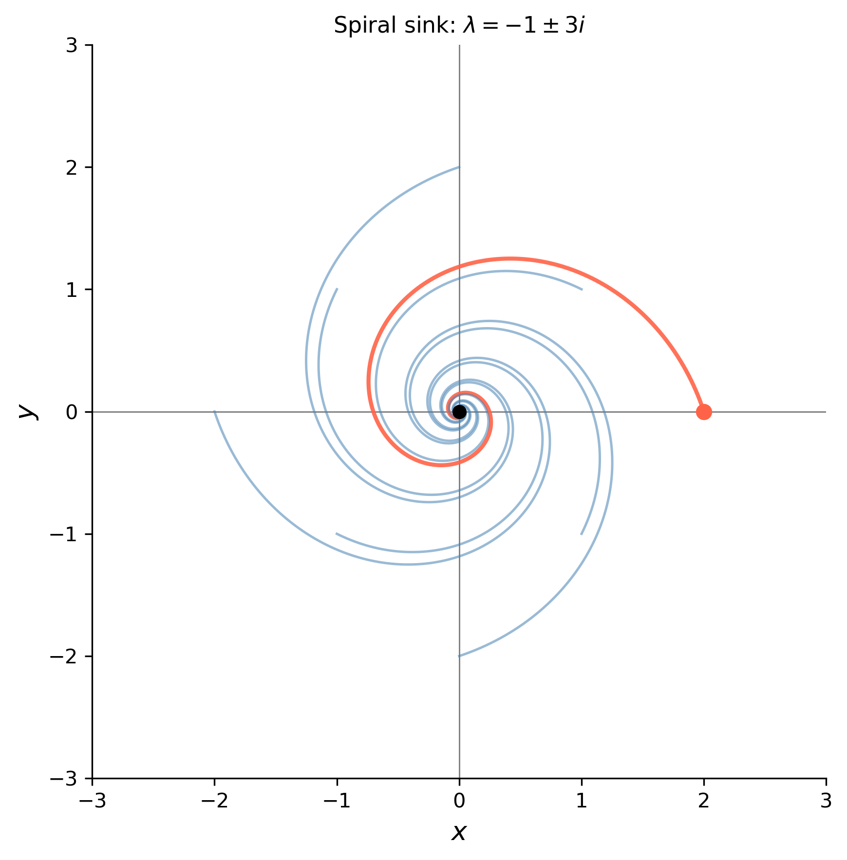
Since \(a = -1 < 0\), trajectories spiral toward the origin: the equilibrium is an asymptotically stable spiral sink.

Tip

Direction of rotation. The sign of the off-diagonal entry \(a_{12}\) in \(A\) helps determine the rotation direction. Here \(a_{12} = -3 < 0\), which produces a clockwise spiral. If \(a_{12} > 0\) the spiral would be counterclockwise. A quick check: at the point \((1,0)\) the velocity is \(A(1,0)^T = (-1, 3)^T\), pointing upward — consistent with counterclockwise motion. (Note the off-diagonal sign here is \(a_{21} = 3 > 0\), consistent with counterclockwise.)

Using SymPy

A4 = sym.Matrix([[-1, -3], [3, -1]])

char4 = A4.charpoly(lam)
display(Math(r'\text{Characteristic polynomial: }\quad'
            + sym.latex(sym.Eq(char4.as_expr(), 0))))

roots4 = sym.solve(char4.as_expr(), lam)
display(Math(r'\lambda = ' + sym.latex(roots4)))

x4 = sym.Function('x')(t)
y4 = sym.Function('y')(t)
sol4 = sym.dsolve([sym.Eq(x4.diff(t), -x4 - 3*y4),
                   sym.Eq(y4.diff(t),  3*x4 - y4)])
for eq in sol4:
    display(Math(sym.latex(eq)))

\(\displaystyle \text{Characteristic polynomial: }\quad\lambda^{2} + 2 \lambda + 10 = 0\)

\(\displaystyle \lambda = \left[ -1 - 3 i, \ -1 + 3 i\right]\)

\(\displaystyle x{\left(t \right)} = - C_{1} e^{- t} \sin{\left(3 t \right)} - C_{2} e^{- t} \cos{\left(3 t \right)}\)

\(\displaystyle y{\left(t \right)} = C_{1} e^{- t} \cos{\left(3 t \right)} - C_{2} e^{- t} \sin{\left(3 t \right)}\)

t_vals = np.linspace(0, 5, 2000)
fig, ax = plt.subplots(figsize=(6, 6))
ax.axhline(0, color='gray', lw=0.7)
ax.axvline(0, color='gray', lw=0.7)

for c1v, c2v, col in [
        ( 2,  0, 'tomato'),
        (-2,  0, 'steelblue'),
        ( 0,  2, 'steelblue'),
        ( 0, -2, 'steelblue'),
        ( 1,  1, 'steelblue'),
        (-1, -1, 'steelblue'),
        ( 1, -1, 'steelblue'),
        (-1,  1, 'steelblue'),
]:
    xc = np.exp(-t_vals)*(c1v*np.cos(3*t_vals) + c2v*np.sin(3*t_vals))
    yc = np.exp(-t_vals)*(c1v*np.sin(3*t_vals) - c2v*np.cos(3*t_vals))
    ax.plot(xc, yc, color=col,
            lw=2.0 if col == 'tomato' else 1.2,
            alpha=0.9 if col == 'tomato' else 0.55)

ax.plot(0, 0, 'ko', ms=6, zorder=5)
ax.plot(2, 0, 'o', color='tomato', ms=7, zorder=5)
ax.set_xlim(-3, 3)
ax.set_ylim(-3, 3)
ax.set_aspect('equal')
ax.set_xlabel(r'$x$', fontsize=13)
ax.set_ylabel(r'$y$', fontsize=13)
ax.set_title(r'Spiral sink: $\lambda = -1 \pm 3i$', fontsize=11)
plt.tight_layout()
plt.show()

Figure 4: Phase portrait for Example 4: asymptotically stable spiral sink with \(\lambda = -1 \pm 3i\). Trajectories spiral inward toward the origin. The tomato orbit starts at \((2,0)\).

---

Example 5 — Purely Imaginary Eigenvalues: Stable Center

Find the general solution of \[ \mathbf{x}' = \begin{pmatrix} 0 & -4 \\ 1 & 0 \end{pmatrix}\mathbf{x}, \] and sketch the phase portrait.

By Hand

Step 1 — Characteristic equation.

\[ \det(A - \lambda I) = \det\begin{pmatrix} -\lambda & -4 \\ 1 & -\lambda \end{pmatrix} = \lambda^2 + 4 = 0. \]

Step 2 — Eigenvalues.

\[ \lambda^2 = -4 \quad\Longrightarrow\quad \lambda = \pm 2i. \]

The eigenvalues are purely imaginary: \(a = 0\), \(b = 2\).

Step 3 — Eigenvector for \(\lambda = 2i\).

Solve \((A - 2iI)\mathbf{v} = \mathbf{0}\):

\[ \begin{pmatrix} -2i & -4 \\ 1 & -2i \end{pmatrix} \begin{pmatrix} v_1 \\ v_2 \end{pmatrix} = \mathbf{0}. \]

Using the second row: \(v_1 - 2iv_2 = 0 \Rightarrow v_1 = 2iv_2\). Choose \(v_2 = 1\), so \(v_1 = 2i\):

\[ \mathbf{v} = \begin{pmatrix} 2i \\ 1 \end{pmatrix} = \underbrace{\begin{pmatrix} 0 \\ 1 \end{pmatrix}}_{\mathbf{w}} + i\underbrace{\begin{pmatrix} 2 \\ 0 \end{pmatrix}}_{\mathbf{z}}. \]

Step 4 — Real-valued fundamental solutions.

With \(a = 0\), the exponential factor \(e^{at} = 1\):

\[ \mathbf{x}_1(t) = \mathbf{w}\cos 2t - \mathbf{z}\sin 2t = \begin{pmatrix} 0 \\ 1 \end{pmatrix}\cos 2t - \begin{pmatrix} 2 \\ 0 \end{pmatrix}\sin 2t = \begin{pmatrix} -2\sin 2t \\ \cos 2t \end{pmatrix}, \]

\[ \mathbf{x}_2(t) = \mathbf{w}\sin 2t + \mathbf{z}\cos 2t = \begin{pmatrix} 0 \\ 1 \end{pmatrix}\sin 2t + \begin{pmatrix} 2 \\ 0 \end{pmatrix}\cos 2t = \begin{pmatrix} 2\cos 2t \\ \sin 2t \end{pmatrix}. \]

Step 5 — General solution.

\[ \boxed{\mathbf{x}(t) = c_1\begin{pmatrix} -2\sin 2t \\ \cos 2t \end{pmatrix} + c_2\begin{pmatrix} 2\cos 2t \\ \sin 2t \end{pmatrix}.} \]

In component form:

\[ x(t) = 2(-c_1 \sin 2t + c_2 \cos 2t), \qquad y(t) = c_1 \cos 2t + c_2 \sin 2t. \]

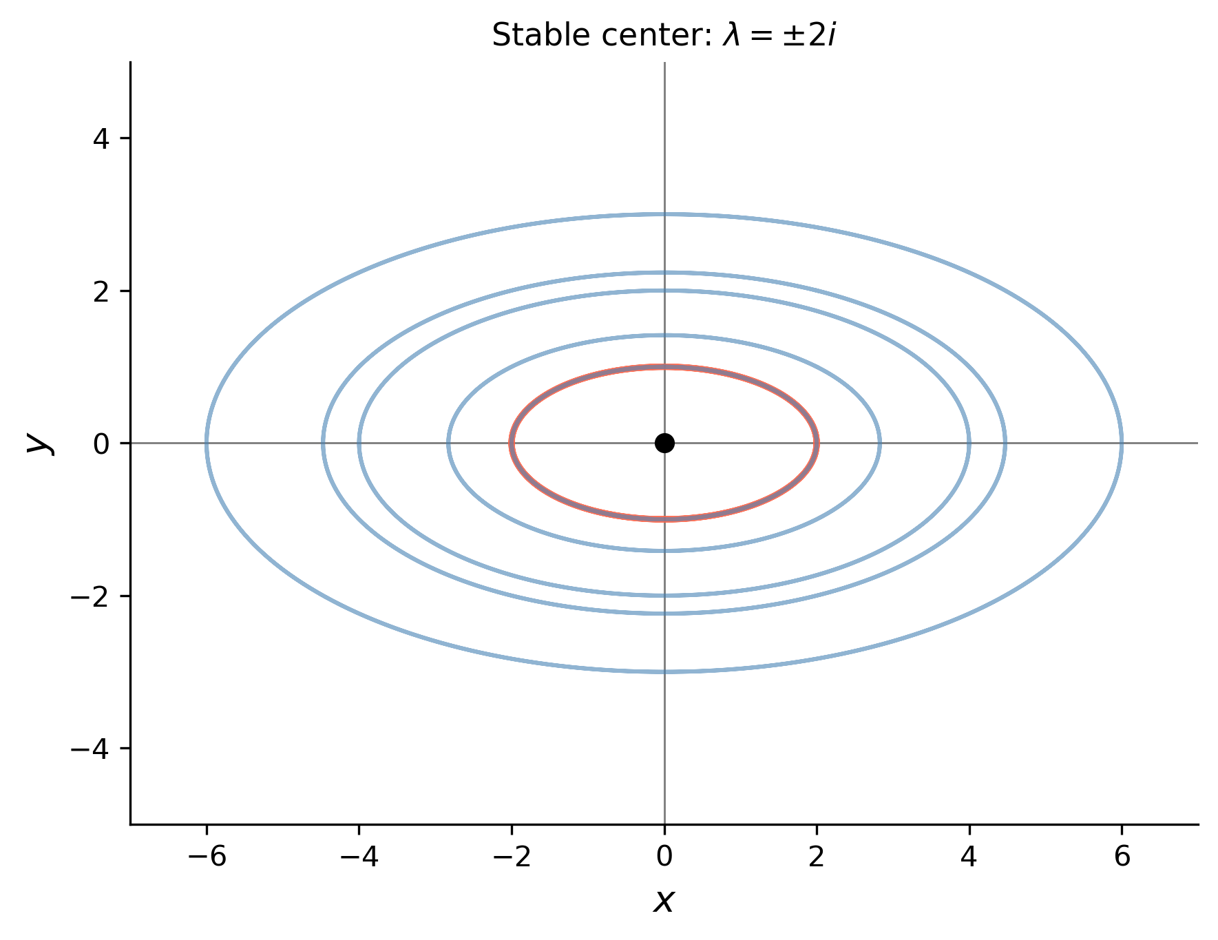
Note that $x(t) = 2y’(t)/2 = $ ; indeed, every solution satisfies \(\tfrac{x^2}{4} + y^2 = c_1^2 + c_2^2 = \text{const}\), confirming that orbits are ellipses centered at the origin. Since \(a = 0\), the amplitude neither grows nor decays; the origin is a stable center.

Note

Center vs. spiral. A center is stable (nearby orbits stay nearby) but not asymptotically stable (orbits do not approach the origin). Any perturbation of the matrix \(A\) that gives \(\operatorname{Re}(\lambda) \neq 0\) destroys the center and produces a spiral, making the center the most structurally fragile equilibrium type.

Using SymPy

A5 = sym.Matrix([[0, -4], [1, 0]])

roots5 = sym.solve(A5.charpoly(lam).as_expr(), lam)
display(Math(r'\lambda = ' + sym.latex(roots5)))

x5 = sym.Function('x')(t)
y5 = sym.Function('y')(t)
sol5 = sym.dsolve([sym.Eq(x5.diff(t), -4*y5),
                   sym.Eq(y5.diff(t),   x5)])
for eq in sol5:
    display(Math(sym.latex(eq)))

\(\displaystyle \lambda = \left[ - 2 i, \ 2 i\right]\)

\(\displaystyle x{\left(t \right)} = - 2 C_{1} \sin{\left(2 t \right)} - 2 C_{2} \cos{\left(2 t \right)}\)

\(\displaystyle y{\left(t \right)} = C_{1} \cos{\left(2 t \right)} - C_{2} \sin{\left(2 t \right)}\)

t_vals = np.linspace(0, 2*np.pi, 1000)
fig, ax = plt.subplots(figsize=(6, 6))
ax.axhline(0, color='gray', lw=0.7)
ax.axvline(0, color='gray', lw=0.7)

for c1v, c2v, col, lw in [
        (0, 1, 'tomato', 2.2),
        (1, 0, 'steelblue', 1.4),
        (0, 2, 'steelblue', 1.4),
        (1, 1, 'steelblue', 1.4),
        (0, 3, 'steelblue', 1.4),
        (2, 1, 'steelblue', 1.4),
]:
    xc = 2*(-c1v*np.sin(2*t_vals) + c2v*np.cos(2*t_vals))
    yc =    c1v*np.cos(2*t_vals)  + c2v*np.sin(2*t_vals)
    ax.plot(xc, yc, color=col, lw=lw, alpha=0.9 if col=='tomato' else 0.6)

ax.plot(0, 0, 'ko', ms=6, zorder=5)
ax.set_xlim(-7, 7)
ax.set_ylim(-5, 5)
ax.set_aspect('equal')
ax.set_xlabel(r'$x$', fontsize=13)
ax.set_ylabel(r'$y$', fontsize=13)
ax.set_title(r'Stable center: $\lambda = \pm 2i$', fontsize=11)
plt.tight_layout()
plt.show()

Figure 5: Phase portrait for Example 5: stable center with \(\lambda = \pm 2i\). Orbits are concentric ellipses satisfying $x^2/4 + y^2 = $ const. The tomato ellipse corresponds to \(c_1=0\), \(c_2=1\).

---

Example 6 — IVP with Complex Eigenvalues

Solve the initial value problem \[ \mathbf{x}' = \begin{pmatrix} 2 & -5 \\ 1 & -2 \end{pmatrix}\mathbf{x}, \qquad \mathbf{x}(0) = \begin{pmatrix} 1 \\ 0 \end{pmatrix}. \]

By Hand

Step 1 — Characteristic equation.

\[ \det(A - \lambda I) = \det\begin{pmatrix} 2-\lambda & -5 \\ 1 & -2-\lambda \end{pmatrix} = (2-\lambda)(-2-\lambda) + 5 = -4 + \lambda^2 + 5 = \lambda^2 + 1 = 0. \]

Step 2 — Eigenvalues.

\[ \lambda = \pm i \quad (a = 0,\; b = 1). \]

The origin is a stable center.

Step 3 — Eigenvector for \(\lambda = i\).

Solve \((A - iI)\mathbf{v} = \mathbf{0}\):

\[ \begin{pmatrix} 2-i & -5 \\ 1 & -2-i \end{pmatrix} \begin{pmatrix} v_1 \\ v_2 \end{pmatrix} = \mathbf{0}. \]

From the second row: \(v_1 + (-2-i)v_2 = 0 \Rightarrow v_1 = (2+i)v_2\). Choose \(v_2 = 1\):

\[ \mathbf{v} = \begin{pmatrix} 2+i \\ 1 \end{pmatrix} = \underbrace{\begin{pmatrix} 2 \\ 1 \end{pmatrix}}_{\mathbf{w}} + i\underbrace{\begin{pmatrix} 1 \\ 0 \end{pmatrix}}_{\mathbf{z}}. \]

Step 4 — Real-valued fundamental solutions (with \(a = 0\), \(b = 1\)):

\[ \mathbf{x}_1(t) = \mathbf{w}\cos t - \mathbf{z}\sin t = \begin{pmatrix} 2\cos t - \sin t \\ \cos t \end{pmatrix}, \]

\[ \mathbf{x}_2(t) = \mathbf{w}\sin t + \mathbf{z}\cos t = \begin{pmatrix} 2\sin t + \cos t \\ \sin t \end{pmatrix}. \]

Step 5 — General solution.

\[ \mathbf{x}(t) = c_1\begin{pmatrix} 2\cos t - \sin t \\ \cos t \end{pmatrix} + c_2\begin{pmatrix} 2\sin t + \cos t \\ \sin t \end{pmatrix}. \]

Step 6 — Apply \(\mathbf{x}(0) = (1, 0)^T\).

At \(t = 0\):

\[ \begin{pmatrix} 2c_1 + c_2 \\ c_1 \end{pmatrix} = \begin{pmatrix} 1 \\ 0 \end{pmatrix}. \]

From the second component: \(c_1 = 0\). Then from the first: \(c_2 = 1\).

Step 7 — Particular solution.

\[ \boxed{\mathbf{x}(t) = \begin{pmatrix} 2\sin t + \cos t \\ \sin t \end{pmatrix}.} \]

In component form:

\[ x(t) = 2\sin t + \cos t, \qquad y(t) = \sin t. \]

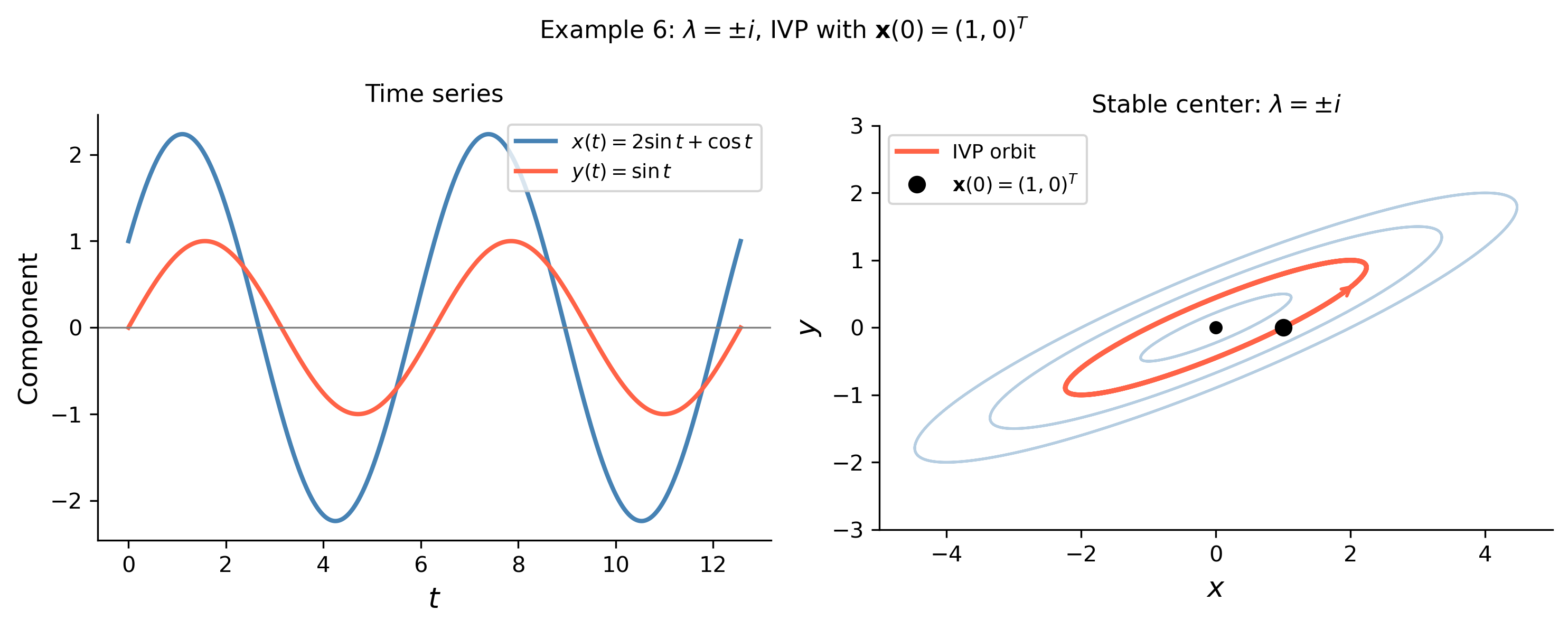
Since \(\lambda = \pm i\) (purely imaginary), the trajectory is a closed periodic orbit of period \(T = 2\pi\).

Tip

Amplitude. Note \(x(t) = 2\sin t + \cos t = \sqrt{5}\sin(t + \phi)\) where \(\phi = \arctan(1/2)\), so \(x\) oscillates with amplitude \(\sqrt{5}\) while \(y\) oscillates with amplitude \(1\). This is consistent with the ellipse \(x^2 - 4xy + 5y^2 = 1\) (obtainable by eliminating \(t\)), centered at the origin.

Using SymPy

A6 = sym.Matrix([[2, -5], [1, -2]])

roots6 = sym.solve(A6.charpoly(lam).as_expr(), lam)
display(Math(r'\lambda = ' + sym.latex(roots6)))

x6 = sym.Function('x')(t)
y6 = sym.Function('y')(t)
sol6_ivp = sym.dsolve(
    [sym.Eq(x6.diff(t),  2*x6 - 5*y6),
     sym.Eq(y6.diff(t),    x6 - 2*y6)],
    ics={x6.subs(t, 0): 1, y6.subs(t, 0): 0}
)
display(Math(r'\text{IVP solution:}'))
for eq in sol6_ivp:
    display(Math(sym.latex(eq)))

\(\displaystyle \lambda = \left[ - i, \ i\right]\)

\(\displaystyle \text{IVP solution:}\)

\(\displaystyle x{\left(t \right)} = 2 \sin{\left(t \right)} + \cos{\left(t \right)}\)

\(\displaystyle y{\left(t \right)} = \sin{\left(t \right)}\)

t_vals = np.linspace(0, 4*np.pi, 1000)
x_sol6 = 2*np.sin(t_vals) + np.cos(t_vals)
y_sol6 = np.sin(t_vals)

fig, axes = plt.subplots(1, 2, figsize=(10, 4))

# Left: time series
ax = axes[0]
ax.plot(t_vals, x_sol6, color='steelblue', lw=2,
        label=r'$x(t) = 2\sin t + \cos t$')
ax.plot(t_vals, y_sol6, color='tomato', lw=2,
        label=r'$y(t) = \sin t$')
ax.axhline(0, color='gray', lw=0.8)
ax.set_xlabel(r'$t$', fontsize=13)
ax.set_ylabel('Component', fontsize=12)
ax.set_title('Time series', fontsize=11)
ax.legend(fontsize=9)

# Right: phase portrait
ax = axes[1]
# Background orbits (other initial conditions)
for c2v in [0.5, 1.5, 2.0]:
    xb = c2v*(2*np.sin(t_vals) + np.cos(t_vals))
    yb = c2v*np.sin(t_vals)
    ax.plot(xb, yb, color='steelblue', lw=1.2, alpha=0.4)

# IVP orbit (c1=0, c2=1)
ax.plot(x_sol6, y_sol6, color='tomato', lw=2.2, label='IVP orbit')
ax.plot(1, 0, 'ko', ms=7, zorder=5, label=r'$\mathbf{x}(0)=(1,0)^T$')
ax.plot(0, 0, 'ko', ms=5, zorder=4)

# Arrow to show direction
idx = 50
ax.annotate('', xy=(x_sol6[idx+5], y_sol6[idx+5]),
            xytext=(x_sol6[idx], y_sol6[idx]),
            arrowprops=dict(arrowstyle='->', color='tomato', lw=1.5))

ax.set_xlim(-5, 5)
ax.set_ylim(-3, 3)
ax.set_aspect('equal')
ax.set_xlabel(r'$x$', fontsize=13)
ax.set_ylabel(r'$y$', fontsize=13)
ax.set_title(r'Stable center: $\lambda = \pm i$', fontsize=11)
ax.legend(fontsize=9)

plt.suptitle(r'Example 6: $\lambda = \pm i$, IVP with $\mathbf{x}(0)=(1,0)^T$',
             fontsize=11)
plt.tight_layout()
plt.show()

Figure 6: Solution of the IVP in Example 6. Left: time series showing \(x(t) = 2\sin t + \cos t\) (steelblue) and \(y(t)=\sin t\) (tomato), both periodic with period \(2\pi\). Right: phase portrait showing the closed elliptical orbit through \((1,0)\).

---

References

Logan, J David. 2015. A First Course in Differential Equations, Third Edition.

TipExpand for Session Info

import sys
print("Python version:", sys.version)
print('\n'.join(f'{m.__name__}=={m.__version__}'
                for m in globals().values()
                if getattr(m, '__version__', None)))

Python version: 3.14.4 | packaged by conda-forge | (main, Apr  8 2026, 02:33:53) [Clang 20.1.8 ]
numpy==2.4.3
sympy==1.14.0
matplotlib==3.10.8

Reuse

CC BY-NC-SA 4.0