Matrices, Linear Systems, and Eigenvalues — Worked Examples

Show the code

# This is a code cell that imports the necessary libraries for our session.
import numpy as np                        # NumPy for numerical computations
import sympy as sym                       # SymPy for symbolic mathematics
import matplotlib as mpl                  # Matplotlib for plotting
import matplotlib.pyplot as plt           # Matplotlib pyplot interface
from IPython.display import Math, display
mpl.rcParams['figure.dpi'] = 150
mpl.rcParams['axes.spines.top'] = False
mpl.rcParams['axes.spines.right'] = False

In this document we work through fully solved examples for the topics covered in Sections 4.2 and 4.3 of the text (Logan 2015):

§4.2 — Matrix algebra (addition, scalar multiplication, matrix multiplication, determinants, inverses) and solving \(2 \times 2\) linear systems \(A\mathbf{x} = \mathbf{b}\) via the inverse matrix and Cramer’s rule.
§4.3 — The eigenvalue problem \(A\mathbf{v} = \lambda\mathbf{v}\): computing eigenvalues from the characteristic equation \(\det(A - \lambda I) = 0\) and finding corresponding eigenvectors, including the cases of real distinct eigenvalues, a repeated eigenvalue, and complex conjugate eigenvalues.

Each example is worked “by hand” first and then verified using NumPy and/or SymPy.

§4.2 Matrix Algebra and Linear Systems

For two \(2\times 2\) matrices \(A\) and \(B\) and a scalar \(k\), recall the basic operations:

\[ (A + B)_{ij} = a_{ij} + b_{ij}, \qquad (kA)_{ij} = k\,a_{ij}, \qquad (AB)_{ij} = \sum_{k=1}^{2} a_{ik}\,b_{kj}. \]

The determinant of \(A = \begin{pmatrix} a & b \\ c & d \end{pmatrix}\) is \(\det A = ad - bc\), and \(A\) is invertible if and only if \(\det A \neq 0\), in which case

\[ A^{-1} = \frac{1}{\det A}\begin{pmatrix} d & -b \\ -c & a \end{pmatrix}. \]

Example 1 — Matrix Arithmetic and the Inverse

Let \[ A = \begin{pmatrix} 2 & -1 \\ 3 & 4 \end{pmatrix}, \qquad B = \begin{pmatrix} 0 & 5 \\ -2 & 1 \end{pmatrix}, \qquad \mathbf{x} = \begin{pmatrix} 1 \\ -3 \end{pmatrix}. \] Compute \(A + B\), \(B - 2A\), \(AB\), \(BA\), \(A^2\), \(B\mathbf{x}\), \(\det A\), and \(A^{-1}\).

By Hand

Step 1 — Matrix addition \(A + B\).

\[ A + B = \begin{pmatrix} 2+0 & -1+5 \\ 3+(-2) & 4+1 \end{pmatrix} = \begin{pmatrix} 2 & 4 \\ 1 & 5 \end{pmatrix}. \]

Step 2 — Scalar combination \(B - 2A\).

\[ B - 2A = \begin{pmatrix} 0-4 & 5-(-2) \\ -2-6 & 1-8 \end{pmatrix} = \begin{pmatrix} -4 & 7 \\ -8 & -7 \end{pmatrix}. \]

Step 3 — Matrix product \(AB\).

\[ AB = \begin{pmatrix} (2)(0)+(-1)(-2) & (2)(5)+(-1)(1) \\ (3)(0)+(4)(-2) & (3)(5)+(4)(1) \end{pmatrix} = \begin{pmatrix} 2 & 9 \\ -8 & 19 \end{pmatrix}. \]

Step 4 — Matrix product \(BA\).

\[ BA = \begin{pmatrix} (0)(2)+(5)(3) & (0)(-1)+(5)(4) \\ (-2)(2)+(1)(3) & (-2)(-1)+(1)(4) \end{pmatrix} = \begin{pmatrix} 15 & 20 \\ -1 & 6 \end{pmatrix}. \]

Note that \(AB \neq BA\); matrix multiplication is in general not commutative.

Step 5 — Matrix square \(A^2 = A \cdot A\).

\[ A^2 = \begin{pmatrix} (2)(2)+(-1)(3) & (2)(-1)+(-1)(4) \\ (3)(2)+(4)(3) & (3)(-1)+(4)(4) \end{pmatrix} = \begin{pmatrix} 1 & -6 \\ 18 & 13 \end{pmatrix}. \]

Step 6 — Matrix-vector product \(B\mathbf{x}\).

\[ B\mathbf{x} = \begin{pmatrix} (0)(1)+(5)(-3) \\ (-2)(1)+(1)(-3) \end{pmatrix} = \begin{pmatrix} -15 \\ -5 \end{pmatrix}. \]

Step 7 — Determinant \(\det A\).

\[ \det A = (2)(4) - (-1)(3) = 8 + 3 = 11. \]

Since \(\det A = 11 \neq 0\), \(A\) is invertible.

Step 8 — Inverse \(A^{-1}\).

\[ A^{-1} = \frac{1}{11}\begin{pmatrix} 4 & 1 \\ -3 & 2 \end{pmatrix} = \begin{pmatrix} \tfrac{4}{11} & \tfrac{1}{11} \\[4pt] -\tfrac{3}{11} & \tfrac{2}{11} \end{pmatrix}. \]

Verification: \(A^{-1}A\) should equal the identity \(I\):

\[ A^{-1}A = \frac{1}{11}\begin{pmatrix} 4 & 1 \\ -3 & 2 \end{pmatrix}\begin{pmatrix} 2 & -1 \\ 3 & 4 \end{pmatrix} = \frac{1}{11}\begin{pmatrix} 11 & 0 \\ 0 & 11 \end{pmatrix} = \begin{pmatrix} 1 & 0 \\ 0 & 1 \end{pmatrix}. \checkmark \]

Using NumPy and SymPy

A = sym.Matrix([[2, -1], [3, 4]])
B = sym.Matrix([[0, 5], [-2, 1]])
x = sym.Matrix([1, -3])

display(Math(r'A + B = ' + sym.latex(A + B)))
display(Math(r'B - 2A = ' + sym.latex(B - 2*A)))
display(Math(r'AB = ' + sym.latex(A * B)))
display(Math(r'BA = ' + sym.latex(B * A)))
display(Math(r'A^2 = ' + sym.latex(A**2)))
display(Math(r'B\mathbf{x} = ' + sym.latex(B * x)))
display(Math(r'\det A = ' + sym.latex(A.det())))
display(Math(r'A^{-1} = ' + sym.latex(A.inv())))

\(\displaystyle A + B = \left[\begin{matrix}2 & 4\\1 & 5\end{matrix}\right]\)

\(\displaystyle B - 2A = \left[\begin{matrix}-4 & 7\\-8 & -7\end{matrix}\right]\)

\(\displaystyle AB = \left[\begin{matrix}2 & 9\\-8 & 19\end{matrix}\right]\)

\(\displaystyle BA = \left[\begin{matrix}15 & 20\\-1 & 6\end{matrix}\right]\)

\(\displaystyle A^2 = \left[\begin{matrix}1 & -6\\18 & 13\end{matrix}\right]\)

\(\displaystyle B\mathbf{x} = \left[\begin{matrix}-15\\-5\end{matrix}\right]\)

\(\displaystyle \det A = 11\)

\(\displaystyle A^{-1} = \left[\begin{matrix}\frac{4}{11} & \frac{1}{11}\\- \frac{3}{11} & \frac{2}{11}\end{matrix}\right]\)

Example 2 — Solving \(A\mathbf{x} = \mathbf{b}\): Inverse Matrix and Cramer’s Rule

Using the matrix \(A\) from Example 1 and \(\mathbf{b} = \begin{pmatrix} 3 \\ -1 \end{pmatrix}\), solve the system \(A\mathbf{x} = \mathbf{b}\) by

multiplying both sides by \(A^{-1}\), and

Cramer’s rule.

By Hand

We have \[ A\mathbf{x} = \mathbf{b} \quad\Longleftrightarrow\quad \begin{pmatrix} 2 & -1 \\ 3 & 4 \end{pmatrix} \begin{pmatrix} x_1 \\ x_2 \end{pmatrix} = \begin{pmatrix} 3 \\ -1 \end{pmatrix}. \]

From Example 1 we know \(\det A = 11\) and \(A^{-1} = \dfrac{1}{11}\begin{pmatrix} 4 & 1 \\ -3 & 2 \end{pmatrix}\).

(a) Inverse-matrix method.

Multiply both sides on the left by \(A^{-1}\):

\[ \mathbf{x} = A^{-1}\mathbf{b} = \frac{1}{11}\begin{pmatrix} 4 & 1 \\ -3 & 2 \end{pmatrix} \begin{pmatrix} 3 \\ -1 \end{pmatrix} = \frac{1}{11}\begin{pmatrix} 4(3)+1(-1) \\ -3(3)+2(-1) \end{pmatrix} = \frac{1}{11}\begin{pmatrix} 11 \\ -11 \end{pmatrix} = \begin{pmatrix} 1 \\ -1 \end{pmatrix}. \]

\[ \boxed{\mathbf{x} = \begin{pmatrix} 1 \\ -1 \end{pmatrix}, \quad\text{i.e., } x_1 = 1,\; x_2 = -1.} \]

(b) Cramer’s rule.

Cramer’s rule states that for a \(2\times 2\) system with \(\det A \neq 0\),

\[ x_1 = \frac{\det A_1}{\det A}, \qquad x_2 = \frac{\det A_2}{\det A}, \]

where \(A_1\) is \(A\) with the first column replaced by \(\mathbf{b}\), and \(A_2\) is \(A\) with the second column replaced by \(\mathbf{b}\).

\[ A_1 = \begin{pmatrix} 3 & -1 \\ -1 & 4 \end{pmatrix}, \quad \det A_1 = (3)(4)-(-1)(-1) = 12 - 1 = 11. \]

\[ A_2 = \begin{pmatrix} 2 & 3 \\ 3 & -1 \end{pmatrix}, \quad \det A_2 = (2)(-1)-(3)(3) = -2 - 9 = -11. \]

Therefore

\[ x_1 = \frac{11}{11} = 1, \qquad x_2 = \frac{-11}{11} = -1. \]

Both methods agree: \[ \boxed{\mathbf{x} = \begin{pmatrix} 1 \\ -1 \end{pmatrix}.} \]

Tip

Geometric interpretation. Each equation \(2x_1 - x_2 = 3\) and \(3x_1 + 4x_2 = -1\) represents a line in the \(x_1 x_2\)-plane. The unique solution \((1, -1)\) is the single point where these two lines intersect. A unique solution exists precisely when \(\det A \neq 0\), which guarantees the lines are not parallel.

Using SymPy

b = sym.Matrix([3, -1])

# Method (a): inverse matrix
x_inv = A.inv() * b
display(Math(r'\mathbf{x} = A^{-1}\mathbf{b} = ' + sym.latex(x_inv)))

# Method (b): Cramer's rule — replace columns manually
A1 = A.copy(); A1[:, 0] = b
A2 = A.copy(); A2[:, 1] = b
x1_cramer = A1.det() / A.det()
x2_cramer = A2.det() / A.det()
display(Math(r"x_1 = \frac{\det A_1}{\det A} = \frac{"
            + sym.latex(A1.det()) + r"}{"
            + sym.latex(A.det()) + r"} = "
            + sym.latex(x1_cramer)))
display(Math(r"x_2 = \frac{\det A_2}{\det A} = \frac{"
            + sym.latex(A2.det()) + r"}{"
            + sym.latex(A.det()) + r"} = "
            + sym.latex(x2_cramer)))

\(\displaystyle \mathbf{x} = A^{-1}\mathbf{b} = \left[\begin{matrix}1\\-1\end{matrix}\right]\)

\(\displaystyle x_1 = \frac{\det A_1}{\det A} = \frac{11}{11} = 1\)

\(\displaystyle x_2 = \frac{\det A_2}{\det A} = \frac{-11}{11} = -1\)

Show the code

x1_vals = np.linspace(-2, 4, 300)

# Line 1: 2x1 - x2 = 3  =>  x2 = 2x1 - 3
line1 = 2*x1_vals - 3

# Line 2: 3x1 + 4x2 = -1  =>  x2 = (-1 - 3x1)/4
line2 = (-1 - 3*x1_vals) / 4

fig, ax = plt.subplots(figsize=(6, 5))
ax.plot(x1_vals, line1, color='steelblue', lw=2,
        label=r'$2x_1 - x_2 = 3$')
ax.plot(x1_vals, line2, color='darkorange', lw=2,
        label=r'$3x_1 + 4x_2 = -1$')
ax.plot(1, -1, 'o', color='tomato', ms=9, zorder=5,
        label=r'Solution $(1,-1)$')
ax.axhline(0, color='gray', lw=0.7)
ax.axvline(0, color='gray', lw=0.7)
ax.set_xlim(-2, 4)
ax.set_ylim(-5, 4)
ax.set_xlabel(r'$x_1$', fontsize=13)
ax.set_ylabel(r'$x_2$', fontsize=13)
ax.set_title(r'$A\mathbf{x} = \mathbf{b}$: intersection of two lines', fontsize=12)
ax.legend(fontsize=10)
plt.tight_layout()
plt.show()

Figure 1: Geometric interpretation of \(A\mathbf{x} = \mathbf{b}\). Each equation defines a line; the unique solution \((1,-1)\) is their intersection (red dot).

§4.3 Eigenvalues and Eigenvectors

Given a square matrix \(A\), a scalar \(\lambda\) is an eigenvalue and a nonzero vector \(\mathbf{v}\) is a corresponding eigenvector if

\[ A\mathbf{v} = \lambda\mathbf{v}. \]

This is equivalent to \(\left(A - \lambda I\right)\mathbf{v} = \mathbf{0}\) having a nontrivial solution, which requires

\[ \det(A - \lambda I) = 0. \]

This is called the characteristic equation. For a \(2\times 2\) matrix it produces a quadratic in \(\lambda\); the nature of the roots (real and distinct, repeated, or complex conjugate) determines the type of eigenpairs.

Example 3 — Real Distinct Eigenvalues

Find the eigenvalues and eigenvectors of \[ A = \begin{pmatrix} 1 & 2 \\ 3 & 2 \end{pmatrix}. \]

By Hand

Step 1 — Set up the characteristic equation.

\[ \det(A - \lambda I) = \det\begin{pmatrix} 1-\lambda & 2 \\ 3 & 2-\lambda \end{pmatrix} = (1-\lambda)(2-\lambda) - (2)(3) = \lambda^2 - 3\lambda + 2 - 6 = \lambda^2 - 3\lambda - 4. \]

Step 2 — Solve \(\lambda^2 - 3\lambda - 4 = 0\).

Factor: \[ (\lambda - 4)(\lambda + 1) = 0 \quad\Longrightarrow\quad \lambda_1 = 4, \quad \lambda_2 = -1. \]

The eigenvalues are real and distinct.

Step 3 — Find the eigenvector for \(\lambda_1 = 4\).

Solve \((A - 4I)\mathbf{v} = \mathbf{0}\):

\[ \begin{pmatrix} 1-4 & 2 \\ 3 & 2-4 \end{pmatrix} \begin{pmatrix} v_1 \\ v_2 \end{pmatrix} = \begin{pmatrix} -3 & 2 \\ 3 & -2 \end{pmatrix} \begin{pmatrix} v_1 \\ v_2 \end{pmatrix} = \mathbf{0}. \]

The two rows are proportional (as expected for a singular matrix), so one equation suffices: \(-3v_1 + 2v_2 = 0\), giving \(v_1 = \tfrac{2}{3}v_2\). Choosing \(v_2 = 3\):

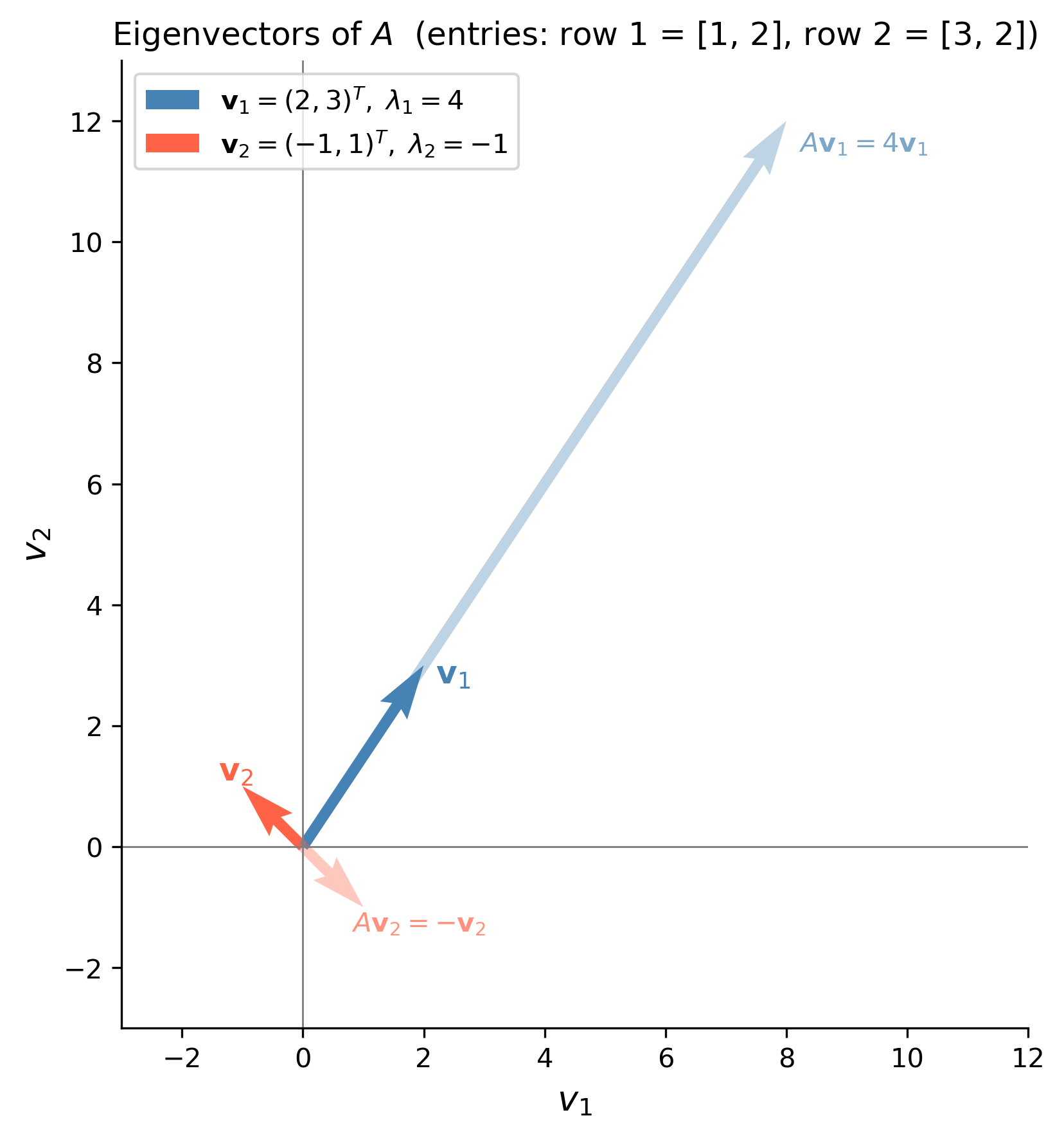
\[ \mathbf{v}_1 = \begin{pmatrix} 2 \\ 3 \end{pmatrix}. \]

Step 4 — Find the eigenvector for \(\lambda_2 = -1\).

Solve \((A + I)\mathbf{v} = \mathbf{0}\):

\[ \begin{pmatrix} 2 & 2 \\ 3 & 3 \end{pmatrix} \begin{pmatrix} v_1 \\ v_2 \end{pmatrix} = \mathbf{0}. \]

From \(2v_1 + 2v_2 = 0\) we get \(v_1 = -v_2\). Choosing \(v_2 = 1\):

\[ \mathbf{v}_2 = \begin{pmatrix} -1 \\ 1 \end{pmatrix}. \]

Summary of eigenpairs:

\[ \boxed{\lambda_1 = 4,\; \mathbf{v}_1 = \begin{pmatrix} 2 \\ 3 \end{pmatrix}; \qquad \lambda_2 = -1,\; \mathbf{v}_2 = \begin{pmatrix} -1 \\ 1 \end{pmatrix}.} \]

Tip

Quick check. The trace of \(A\) equals the sum of the eigenvalues: \(\text{tr}(A) = 1 + 2 = 3 = 4 + (-1) = \lambda_1 + \lambda_2\). \(\checkmark\)

The determinant of \(A\) equals the product of the eigenvalues: \(\det A = (1)(2)-(2)(3) = -4 = (4)(-1) = \lambda_1\lambda_2\). \(\checkmark\)

These trace-determinant identities provide a fast consistency check.

Using NumPy and SymPy

A3 = sym.Matrix([[1, 2], [3, 2]])
lam = sym.Symbol('lambda')

char_poly = A3.charpoly(lam)
display(Math(r'\text{Characteristic polynomial: }\quad'
            + sym.latex(sym.Eq(char_poly.as_expr(), 0))))

eigvals = sym.solve(char_poly.as_expr(), lam)
display(Math(r'\text{Eigenvalues: }\quad \lambda = ' + sym.latex(eigvals)))

for ev in eigvals:
    evecs = (A3 - ev*sym.eye(2)).nullspace()
    display(Math(r'\lambda = ' + sym.latex(ev)
                 + r',\quad \mathbf{v} = ' + sym.latex(evecs[0])))

\(\displaystyle \text{Characteristic polynomial: }\quad\lambda^{2} - 3 \lambda - 4 = 0\)

\(\displaystyle \text{Eigenvalues: }\quad \lambda = \left[ -1, \ 4\right]\)

\(\displaystyle \lambda = -1,\quad \mathbf{v} = \left[\begin{matrix}-1\\1\end{matrix}\right]\)

\(\displaystyle \lambda = 4,\quad \mathbf{v} = \left[\begin{matrix}\frac{2}{3}\\1\end{matrix}\right]\)

Show the code

A3_np = np.array([[1, 2], [3, 2]], dtype=float)
v1 = np.array([2, 3], dtype=float)
v2 = np.array([-1, 1], dtype=float)
v1n = v1 / np.linalg.norm(v1)
v2n = v2 / np.linalg.norm(v2)

fig, ax = plt.subplots(figsize=(6, 6))
ax.axhline(0, color='gray', lw=0.7)
ax.axvline(0, color='gray', lw=0.7)

# Eigenvectors
ax.quiver(0, 0, v1[0], v1[1], angles='xy', scale_units='xy', scale=1,
          color='steelblue', width=0.012, label=r'$\mathbf{v}_1=(2,3)^T,\;\lambda_1=4$')
ax.quiver(0, 0, v2[0], v2[1], angles='xy', scale_units='xy', scale=1,
          color='tomato', width=0.012, label=r'$\mathbf{v}_2=(-1,1)^T,\;\lambda_2=-1$')

# A*v1 and A*v2 (should be lambda*v)
Av1 = A3_np @ v1   # = 4*v1
Av2 = A3_np @ v2   # = -1*v2
ax.quiver(0, 0, Av1[0], Av1[1], angles='xy', scale_units='xy', scale=1,
          color='steelblue', alpha=0.35, width=0.012, linestyle='dashed')
ax.quiver(0, 0, Av2[0], Av2[1], angles='xy', scale_units='xy', scale=1,
          color='tomato', alpha=0.35, width=0.012, linestyle='dashed')

# Annotations
ax.annotate(r'$\mathbf{v}_1$', xy=v1, xytext=(2.2, 2.7), fontsize=12,
            color='steelblue')
ax.annotate(r'$A\mathbf{v}_1 = 4\mathbf{v}_1$', xy=Av1,
            xytext=(8.2, 11.5), fontsize=10, color='steelblue', alpha=0.7)
ax.annotate(r'$\mathbf{v}_2$', xy=v2, xytext=(-1.4, 1.1), fontsize=12,
            color='tomato')
ax.annotate(r'$A\mathbf{v}_2 = -\mathbf{v}_2$', xy=Av2,
            xytext=(0.8, -1.4), fontsize=10, color='tomato', alpha=0.7)

ax.set_xlim(-3, 12)
ax.set_ylim(-3, 13)
ax.set_aspect('equal')
ax.set_xlabel(r'$v_1$', fontsize=13)
ax.set_ylabel(r'$v_2$', fontsize=13)
ax.set_title(r'Eigenvectors of $A$  (entries: row 1 = [1, 2], row 2 = [3, 2])',
             fontsize=12)
ax.legend(fontsize=10, loc='upper left')
plt.tight_layout()
plt.show()

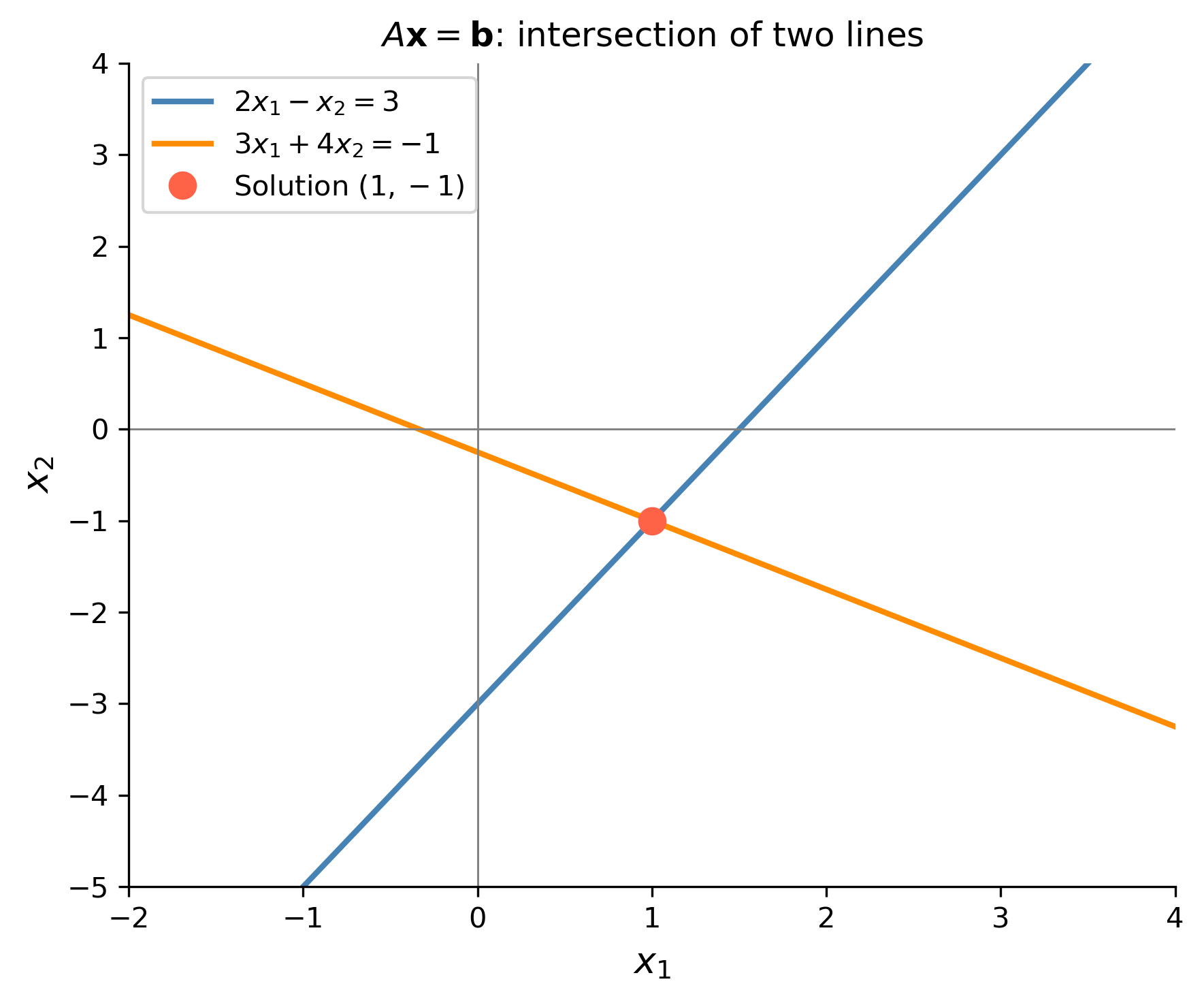
Figure 2: Eigenvectors of \(A\) plotted from the origin (scaled for visibility). The vector \(\mathbf{v}_1 = (2,3)^T\) corresponds to \(\lambda_1 = 4\) and \(\mathbf{v}_2 = (-1,1)^T\) to \(\lambda_2 = -1\). Arrows show how \(A\) maps each eigenvector to a scalar multiple of itself.

Example 4 — Repeated Eigenvalue

Find the eigenvalues and eigenvectors of \[ A = \begin{pmatrix} -3 & 1 \\ 0 & -3 \end{pmatrix}. \]

By Hand

Step 1 — Characteristic equation.

\[ \det(A - \lambda I) = \det\begin{pmatrix} -3-\lambda & 1 \\ 0 & -3-\lambda \end{pmatrix} = (-3-\lambda)^2 = 0. \]

Step 2 — Solve for \(\lambda\).

\[ (-3-\lambda)^2 = 0 \quad\Longrightarrow\quad \lambda = -3 \text{ (repeated eigenvalue)}. \]

Step 3 — Find the eigenvectors for \(\lambda = -3\).

Solve \((A - (-3)I)\mathbf{v} = \mathbf{0}\), i.e., \((A + 3I)\mathbf{v} = \mathbf{0}\):

\[ \begin{pmatrix} 0 & 1 \\ 0 & 0 \end{pmatrix} \begin{pmatrix} v_1 \\ v_2 \end{pmatrix} = \mathbf{0} \quad\Longrightarrow\quad v_2 = 0, \quad v_1 \text{ free}. \]

Choosing \(v_1 = 1\):

\[ \mathbf{v} = \begin{pmatrix} 1 \\ 0 \end{pmatrix}. \]

\[ \boxed{\lambda = -3 \text{ (repeated)}, \quad \mathbf{v} = \begin{pmatrix} 1 \\ 0 \end{pmatrix}.} \]

Note

Defective matrix. Although \(\lambda = -3\) is a double root of the characteristic equation (algebraic multiplicity 2), there is only one linearly independent eigenvector (geometric multiplicity 1). A matrix with this property is called defective. When solving the corresponding linear system \(\mathbf{x}' = A\mathbf{x}\), a second independent solution must be constructed using a generalized eigenvector — a vector \(\mathbf{w}\) satisfying \((A - \lambda I)\mathbf{w} = \mathbf{v}\) rather than \((A - \lambda I)\mathbf{w} = \mathbf{0}\).

Using SymPy

A4 = sym.Matrix([[-3, 1], [0, -3]])

char_poly4 = A4.charpoly(lam)
display(Math(r'\text{Characteristic polynomial: }\quad'
            + sym.latex(sym.Eq(char_poly4.as_expr(), 0))))

display(Math(r'\text{Eigenvalues: }' + sym.latex(A4.eigenvals())))

for ev, mult, evecs in A4.eigenvects():
    display(Math(r'\lambda = ' + sym.latex(ev)
                 + r'\;(\text{multiplicity } ' + str(mult) + r'),\quad'
                 + r'\mathbf{v} = ' + sym.latex(evecs[0])))

\(\displaystyle \text{Characteristic polynomial: }\quad\lambda^{2} + 6 \lambda + 9 = 0\)

\(\displaystyle \text{Eigenvalues: }\left\{ -3 : 2\right\}\)

\(\displaystyle \lambda = -3\;(\text{multiplicity } 2),\quad\mathbf{v} = \left[\begin{matrix}1\\0\end{matrix}\right]\)

Example 5 — Complex Conjugate Eigenvalues

Find the eigenvalues and eigenvectors of \[ A = \begin{pmatrix} 1 & -5 \\ 2 & -3 \end{pmatrix}. \]

By Hand

Step 1 — Characteristic equation.

\[ \det(A - \lambda I) = \det\begin{pmatrix} 1-\lambda & -5 \\ 2 & -3-\lambda \end{pmatrix} = (1-\lambda)(-3-\lambda) - (-5)(2). \]

Expand:

\[ = -3 - \lambda + 3\lambda + \lambda^2 + 10 = \lambda^2 + 2\lambda + 7. \]

Step 2 — Solve \(\lambda^2 + 2\lambda + 7 = 0\).

Using the quadratic formula:

\[ \lambda = \frac{-2 \pm \sqrt{4 - 28}}{2} = \frac{-2 \pm \sqrt{-24}}{2} = \frac{-2 \pm 2i\sqrt{6}}{2} = -1 \pm i\sqrt{6}. \]

The eigenvalues are complex conjugates \(\lambda = \alpha \pm \beta i\) with \(\alpha = -1\) and \(\beta = \sqrt{6}\).

Step 3 — Find the eigenvector for \(\lambda_1 = -1 + i\sqrt{6}\).

Solve \((A - \lambda_1 I)\mathbf{v} = \mathbf{0}\):

\[ \begin{pmatrix} 1 - (-1+i\sqrt{6}) & -5 \\ 2 & -3-(-1+i\sqrt{6}) \end{pmatrix} = \begin{pmatrix} 2 - i\sqrt{6} & -5 \\ 2 & -2 - i\sqrt{6} \end{pmatrix}. \]

Use the first row: \((2 - i\sqrt{6})\,v_1 - 5v_2 = 0\), so \(v_1 = \dfrac{5}{2-i\sqrt{6}}\,v_2\).

Choose \(v_2 = 2 - i\sqrt{6}\):

\[ \mathbf{v}_1 = \begin{pmatrix} 5 \\ 2 - i\sqrt{6} \end{pmatrix}. \]

The eigenvector for \(\lambda_2 = -1 - i\sqrt{6}\) is the complex conjugate:

\[ \mathbf{v}_2 = \begin{pmatrix} 5 \\ 2 + i\sqrt{6} \end{pmatrix}. \]

\[ \boxed{\lambda_{1,2} = -1 \pm i\sqrt{6},\quad \mathbf{v}_{1,2} = \begin{pmatrix} 5 \\ 2 \mp i\sqrt{6} \end{pmatrix}.} \]

Tip

Stability from the sign of \(\alpha\). Because \(\alpha = -1 < 0\), the equilibrium \(\mathbf{x}^* = \mathbf{0}\) of the associated system \(\mathbf{x}' = A\mathbf{x}\) is asymptotically stable (a spiral sink): all trajectories spiral toward the origin as \(t \to +\infty\). If \(\alpha > 0\) the origin would be a spiral source (unstable), and if \(\alpha = 0\) trajectories would be closed ellipses (stable center).

Using SymPy

A5 = sym.Matrix([[1, -5], [2, -3]])

char_poly5 = A5.charpoly(lam)
display(Math(r'\text{Characteristic polynomial: }\quad'
            + sym.latex(sym.Eq(char_poly5.as_expr(), 0))))

roots5 = sym.solve(char_poly5.as_expr(), lam)
display(Math(r'\text{Eigenvalues: }\quad \lambda = ' + sym.latex(roots5)))

for ev, mult, evecs in A5.eigenvects():
    display(Math(r'\lambda = ' + sym.latex(ev)
                 + r',\quad \mathbf{v} = ' + sym.latex(evecs[0])))

\(\displaystyle \text{Characteristic polynomial: }\quad\lambda^{2} + 2 \lambda + 7 = 0\)

\(\displaystyle \text{Eigenvalues: }\quad \lambda = \left[ -1 - \sqrt{6} i, \ -1 + \sqrt{6} i\right]\)

\(\displaystyle \lambda = -1 - \sqrt{6} i,\quad \mathbf{v} = \left[\begin{matrix}1 - \frac{\sqrt{6} i}{2}\\1\end{matrix}\right]\)

\(\displaystyle \lambda = -1 + \sqrt{6} i,\quad \mathbf{v} = \left[\begin{matrix}1 + \frac{\sqrt{6} i}{2}\\1\end{matrix}\right]\)

Example 6 — Eigenvalues Depending on a Parameter

Let \[ A(\beta) = \begin{pmatrix} -1 & \beta \\ -1 & -1 \end{pmatrix}, \qquad \beta \in \mathbb{R}. \] Find the eigenvalues as functions of \(\beta\) and determine the values of \(\beta\) for which the eigenvalues are (i) real and distinct, (ii) real and repeated, and (iii) complex conjugates.

By Hand

Step 1 — Characteristic equation.

\[ \det(A - \lambda I) = \det\begin{pmatrix} -1-\lambda & \beta \\ -1 & -1-\lambda \end{pmatrix} = (-1-\lambda)^2 - \beta(-1) = (-1-\lambda)^2 + \beta. \]

Expanding:

\[ \lambda^2 + 2\lambda + 1 + \beta = 0. \]

Step 2 — Solve using the quadratic formula.

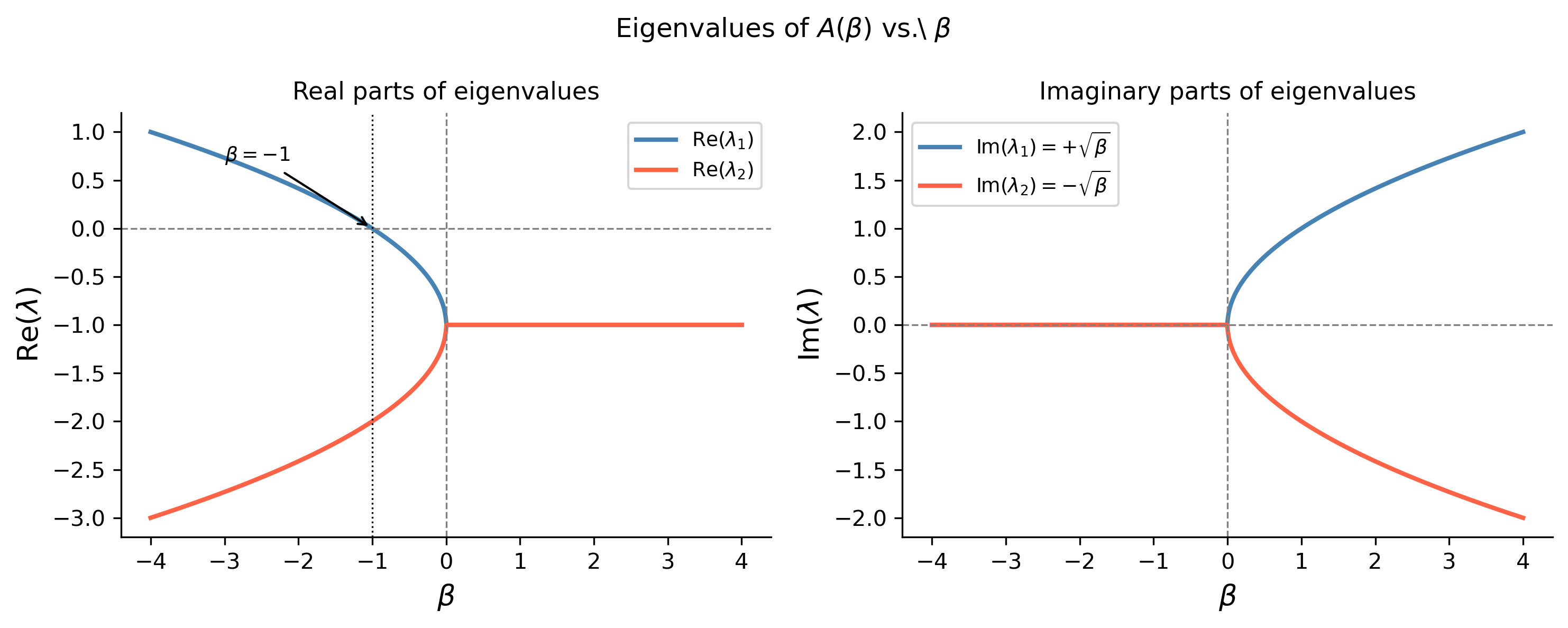
\[ \lambda = \frac{-2 \pm \sqrt{4 - 4(1+\beta)}}{2} = \frac{-2 \pm \sqrt{-4\beta}}{2} = -1 \pm \sqrt{-\beta}. \]

The discriminant is \(\Delta = -4\beta\).

Step 3 — Classify by the sign of \(\beta\).

Condition	Discriminant \(\Delta\)	Eigenvalue type	Stability
\(\beta < 0\)	\(\Delta = -4\beta > 0\)	Real, distinct: \(\lambda = -1 \pm \sqrt{-\beta}\)	Depends on signs of \(\lambda_{1,2}\)
\(\beta = 0\)	\(\Delta = 0\)	Real, repeated: \(\lambda = -1\)	Asymptotically stable
\(\beta > 0\)	\(\Delta = -4\beta < 0\)	Complex: \(\lambda = -1 \pm i\sqrt{\beta}\)	Asymptotically stable (spiral sink, \(\alpha = -1 < 0\))

For \(\beta < 0\): note \(\lambda_1 = -1 + \sqrt{-\beta}\) and \(\lambda_2 = -1 - \sqrt{-\beta}\). Since \(\sqrt{-\beta} > 0\), the sign of \(\lambda_1\) depends on whether \(\sqrt{-\beta}\) exceeds \(1\), i.e., whether \(-\beta > 1\), i.e., whether \(\beta < -1\):

\(-1 < \beta < 0\): both eigenvalues are negative (stable node).
\(\beta = -1\): \(\lambda_1 = 0\), \(\lambda_2 = -2\) (borderline — non-isolated equilibrium).
\(\beta < -1\): \(\lambda_1 > 0 > \lambda_2\) (unstable saddle point).

\[ \boxed{ \lambda(\beta) = -1 \pm \sqrt{-\beta}. } \]

Note

Bifurcation at \(\beta = 0\). As \(\beta\) increases through \(0\) the eigenvalues transition from real to complex. This is a qualitative change in the phase portrait of \(\mathbf{x}' = A\mathbf{x}\): orbits change from node-like (approaching the origin along straight lines) to spiral-like (winding toward the origin). The value \(\beta = 0\) at which this transition occurs is called a bifurcation value.

Using SymPy

beta = sym.Symbol('beta', real=True)

A6 = sym.Matrix([[-1, beta], [-1, -1]])
char_poly6 = A6.charpoly(lam)
display(Math(r'\text{Characteristic polynomial: }\quad'
            + sym.latex(sym.Eq(char_poly6.as_expr(), 0))))

roots6 = sym.solve(char_poly6.as_expr(), lam)
display(Math(r'\lambda(\beta) = ' + sym.latex(roots6)))

\(\displaystyle \text{Characteristic polynomial: }\quad\beta + \lambda^{2} + 2 \lambda + 1 = 0\)

\(\displaystyle \lambda(\beta) = \left[ - \sqrt{- \beta} - 1, \ \sqrt{- \beta} - 1\right]\)

Show the code

beta_vals = np.linspace(-4, 4, 800)

# Eigenvalue formula: -1 ± sqrt(-beta)
# For beta < 0: sqrt(-beta) is real
# For beta > 0: sqrt(-beta) = i*sqrt(beta) -- complex

real_part_plus  = np.where(beta_vals <= 0,
                           -1 + np.sqrt(np.maximum(-beta_vals, 0)),
                           -1 * np.ones_like(beta_vals))
real_part_minus = np.where(beta_vals <= 0,
                           -1 - np.sqrt(np.maximum(-beta_vals, 0)),
                           -1 * np.ones_like(beta_vals))
imag_part = np.where(beta_vals >= 0,
                     np.sqrt(np.maximum(beta_vals, 0)),
                     np.zeros_like(beta_vals))

fig, axes = plt.subplots(1, 2, figsize=(10, 4))

# Left: real parts
ax = axes[0]
ax.plot(beta_vals, real_part_plus,  color='steelblue', lw=2,
        label=r'$\operatorname{Re}(\lambda_1)$')
ax.plot(beta_vals, real_part_minus, color='tomato', lw=2,
        label=r'$\operatorname{Re}(\lambda_2)$')
ax.axvline(0, color='gray', lw=0.8, ls='--')
ax.axhline(0, color='gray', lw=0.8, ls='--')
ax.axvline(-1, color='black', lw=0.8, ls=':')
ax.set_xlabel(r'$\beta$', fontsize=13)
ax.set_ylabel(r'$\operatorname{Re}(\lambda)$', fontsize=13)
ax.set_title('Real parts of eigenvalues', fontsize=11)
ax.legend(fontsize=9)
ax.annotate(r'$\beta=-1$', xy=(-1, 0), xytext=(-3, 0.7), fontsize=9,
            arrowprops=dict(arrowstyle='->', color='black'))

# Right: imaginary parts
ax = axes[1]
ax.plot(beta_vals,  imag_part, color='steelblue', lw=2,
        label=r'$\operatorname{Im}(\lambda_1) = +\sqrt{\beta}$')
ax.plot(beta_vals, -imag_part, color='tomato', lw=2,
        label=r'$\operatorname{Im}(\lambda_2) = -\sqrt{\beta}$')
ax.axvline(0, color='gray', lw=0.8, ls='--')
ax.axhline(0, color='gray', lw=0.8, ls='--')
ax.set_xlabel(r'$\beta$', fontsize=13)
ax.set_ylabel(r'$\operatorname{Im}(\lambda)$', fontsize=13)
ax.set_title('Imaginary parts of eigenvalues', fontsize=11)
ax.legend(fontsize=9)

plt.suptitle(r'Eigenvalues of $A(\beta)$ vs.\ $\beta$', fontsize=12)
plt.tight_layout()
plt.show()

Figure 3: Real part (solid) and imaginary part (dashed) of the eigenvalues \(\lambda(\beta) = -1 \pm \sqrt{-\beta}\) as functions of \(\beta\). For \(\beta < 0\) the eigenvalues are real; for \(\beta > 0\) they are complex conjugates with real part \(-1\). The transition occurs at \(\beta = 0\).

References

Logan, J David. 2015. A First Course in Differential Equations, Third Edition.

Expand for Session Info

import sys
print("Python version:", sys.version)
print('\n'.join(f'{m.__name__}=={m.__version__}'
                for m in globals().values()
                if getattr(m, '__version__', None)))

Python version: 3.14.4 | packaged by conda-forge | (main, Apr  8 2026, 02:33:53) [Clang 20.1.8 ]
numpy==2.4.3
sympy==1.14.0
matplotlib==3.10.8

Reuse

CC BY-NC-SA 4.0