Nonlinear Systems — Worked Examples

# This is a code cell that imports the necessary libraries for our session.
import numpy as np                        # NumPy for numerical computations
import sympy as sym                       # SymPy for symbolic mathematics
import matplotlib as mpl                  # Matplotlib for plotting
import matplotlib.pyplot as plt           # Matplotlib pyplot interface
from scipy.integrate import solve_ivp     # SciPy ODE solver
from IPython.display import Math, display
mpl.rcParams['figure.dpi'] = 150
mpl.rcParams['axes.spines.top'] = False
mpl.rcParams['axes.spines.right'] = False

In this document we work through fully solved examples for the topics covered in Sections 5.1 and 5.2 of the text (Logan 2015):

• §5.1 — Linearization of nonlinear systems: finding equilibria of \(\mathbf{x}' = \mathbf{F}(\mathbf{x})\), classifying them via the Jacobian matrix \(J = D\mathbf{F}\), sketching nullclines and phase portraits, and analyzing systems with a parameter. We also illustrate finding exact orbit equations via \(dy/dx\).
• §5.2 — Nonlinear mechanics: converting second-order equations to first-order systems, finding potential energy functions, writing conservation-of-energy laws, plotting constant-energy orbits in the phase plane, and the nonlinear pendulum.

Each example is worked “by hand” first and then verified or illustrated using NumPy, SymPy, and SciPy.

---

§5.1 Linearization of Nonlinear Systems

Given a nonlinear autonomous system \(x' = F(x,y)\), \(y' = G(x,y)\), an equilibrium (critical point) is a point \((x^*, y^*)\) where \(F = G = 0\). Near each isolated equilibrium the behavior is approximated by the linearized system

\[ \mathbf{u}' = J(x^*, y^*)\,\mathbf{u}, \qquad J = \begin{pmatrix} F_x & F_y \\ G_x & G_y \end{pmatrix}, \]

where \(\mathbf{u} = \mathbf{x} - \mathbf{x}^*\) and \(J(x^*,y^*)\) is the Jacobian evaluated at the equilibrium. The eigenvalues of \(J\) classify the equilibrium type and stability, provided the equilibrium is hyperbolic (no eigenvalue has zero real part).

---

Example 1 — Full Nonlinear Analysis: Two Equilibria

For the nonlinear system \[ x' = x - xy, \qquad y' = -y + x^2, \] (a) find all equilibria, (b) classify each via the Jacobian, (c) find and sketch the nullclines, and (d) sketch the phase portrait.

By Hand

Step 1 — Find the equilibria.

Set \(F = x - xy = x(1-y) = 0\) and \(G = -y + x^2 = 0\) simultaneously.

From \(F = 0\): either \(x = 0\) or \(y = 1\).

• Case \(x = 0\): \(G = -y + 0 = 0 \Rightarrow y = 0\). Equilibrium: \((0, 0)\).
• Case \(y = 1\): \(G = -1 + x^2 = 0 \Rightarrow x = \pm 1\). Equilibria: \((1, 1)\) and \((-1, 1)\).

There are three equilibria: \((0,0)\), \((1,1)\), \((-1,1)\).

Step 2 — Compute the Jacobian.

\[ J = \begin{pmatrix} \partial F/\partial x & \partial F/\partial y \\ \partial G/\partial x & \partial G/\partial y \end{pmatrix} = \begin{pmatrix} 1 - y & -x \\ 2x & -1 \end{pmatrix}. \]

Step 3 — Classify each equilibrium.

At \((0, 0)\):

\[ J(0,0) = \begin{pmatrix} 1 & 0 \\ 0 & -1 \end{pmatrix}. \]

Eigenvalues: \(\lambda_1 = 1\), \(\lambda_2 = -1\) (read directly from the diagonal). Since the eigenvalues are real with opposite signs, \((0,0)\) is an unstable saddle point.

At \((1, 1)\):

\[ J(1,1) = \begin{pmatrix} 1-1 & -1 \\ 2 & -1 \end{pmatrix} = \begin{pmatrix} 0 & -1 \\ 2 & -1 \end{pmatrix}. \]

Characteristic equation: \[ \det(J - \lambda I) = \lambda(\lambda+1) + 2 = \lambda^2 + \lambda + 2 = 0. \] \[ \lambda = \frac{-1 \pm \sqrt{1 - 8}}{2} = \frac{-1 \pm i\sqrt{7}}{2}. \]

Real part \(\alpha = -\tfrac{1}{2} < 0\), so \((1,1)\) is an asymptotically stable spiral sink.

At \((-1, 1)\):

\[ J(-1,1) = \begin{pmatrix} 0 & 1 \\ -2 & -1 \end{pmatrix}. \]

Characteristic equation: \[ \lambda^2 + \lambda + 2 = 0 \quad\Longrightarrow\quad \lambda = \frac{-1 \pm i\sqrt{7}}{2}. \]

Same eigenvalues as \((1,1)\), so \((-1,1)\) is also an asymptotically stable spiral sink.

Step 4 — Nullclines.

• \(x\)-nullcline (\(x' = 0\)): \(x(1 - y) = 0\), i.e. \(x = 0\) or \(y = 1\).
• \(y\)-nullcline (\(y' = 0\)): \(-y + x^2 = 0\), i.e. \(y = x^2\) (a parabola).

\[ \boxed{\text{Equilibria: } (0,0) \text{ saddle};\quad (1,1),(-1,1) \text{ stable spiral sinks.}} \]

Tip

Reading stability from \(\tau\) and \(\delta\). For the Jacobian at \((1,1)\): \(\tau = \operatorname{tr}(J) = 0 + (-1) = -1 < 0\) and \(\delta = \det(J) = (0)(-1) - (-1)(2) = 2 > 0\). The discriminant \(\tau^2 - 4\delta = 1 - 8 = -7 < 0\), confirming complex eigenvalues with negative real part — a spiral sink. This trace-determinant check is often faster than computing eigenvalues explicitly.

Using SymPy

x, y = sym.symbols('x y')

F1 = x*(1 - y)
G1 = -y + x**2

# Jacobian
J1 = sym.Matrix([[sym.diff(F1,x), sym.diff(F1,y)],
                 [sym.diff(G1,x), sym.diff(G1,y)]])
display(Math(r'J = ' + sym.latex(J1)))

# Equilibria
equil1 = sym.solve([F1, G1], [x, y])
display(Math(r'\text{Equilibria: }' + sym.latex(equil1)))

# Classify each
for pt in equil1:
    Jpt = J1.subs([(x, pt[0]), (y, pt[1])])
    eigs = Jpt.eigenvals()
    tau  = Jpt.trace()
    delta = Jpt.det()
    display(Math(r'(' + sym.latex(pt[0]) + r',' + sym.latex(pt[1]) + r'):\quad'
                 + r'\tau=' + sym.latex(tau)
                 + r',\;\delta=' + sym.latex(delta)
                 + r',\;\lambda=' + sym.latex(list(eigs.keys()))))

\(\displaystyle J = \left[\begin{matrix}1 - y & - x\\2 x & -1\end{matrix}\right]\)

\(\displaystyle \text{Equilibria: }\left[ \left( -1, \ 1\right), \ \left( 0, \ 0\right), \ \left( 1, \ 1\right)\right]\)

\(\displaystyle (-1,1):\quad\tau=-1,\;\delta=2,\;\lambda=\left[ - \frac{1}{2} - \frac{\sqrt{7} i}{2}, \ - \frac{1}{2} + \frac{\sqrt{7} i}{2}\right]\)

\(\displaystyle (0,0):\quad\tau=0,\;\delta=-1,\;\lambda=\left[ 1, \ -1\right]\)

\(\displaystyle (1,1):\quad\tau=-1,\;\delta=2,\;\lambda=\left[ - \frac{1}{2} - \frac{\sqrt{7} i}{2}, \ - \frac{1}{2} + \frac{\sqrt{7} i}{2}\right]\)

def sys1(t, state):
    xv, yv = state
    return [xv*(1 - yv), -yv + xv**2]

fig, ax = plt.subplots(figsize=(7, 6))

# Nullclines
xr = np.linspace(-2.5, 2.5, 400)
ax.axvline(0,   color='steelblue',  lw=1.6, ls='--', label=r"$x'=0$: $x=0$")
ax.axhline(1,   color='steelblue',  lw=1.6, ls='--', label=r"$x'=0$: $y=1$")
ax.plot(xr, xr**2, color='darkorange', lw=1.6, ls='--', label=r"$y'=0$: $y=x^2$")

# Direction field
X, Y = np.meshgrid(np.linspace(-2.5, 2.5, 20), np.linspace(-0.5, 3.0, 20))
U = X*(1 - Y)
V = -Y + X**2
spd = np.sqrt(U**2 + V**2)
spd[spd == 0] = 1
ax.quiver(X, Y, U/spd, V/spd, alpha=0.3, color='gray',
          scale=25, width=0.003)

# Trajectories from several initial conditions
ic_list = [
    (0.1, 0.1), (-0.1, 0.1), (0.5, 2.5), (-0.5, 2.5),
    (1.8, 0.2), (-1.8, 0.2), (0.3, 2.8), (-0.3, 2.8),
    (1.5, 2.5), (-1.5, 2.5), (2.0, 1.5), (-2.0, 1.5),
    (0.8, 0.1), (-0.8, 0.1),
]
for x0, y0 in ic_list:
    sol = solve_ivp(sys1, [0, 12], [x0, y0], max_step=0.05,
                    dense_output=True)
    ts = np.linspace(0, 12, 1200)
    xs, ys = sol.sol(ts)
    mask = (np.abs(xs) < 2.6) & (np.abs(ys) < 3.1) & (ys > -0.6)
    ax.plot(xs[mask], ys[mask], color='steelblue', lw=1.0, alpha=0.55)

# Equilibria
ax.plot(0,  0, 's', color='tomato',    ms=9, zorder=6, label='Saddle $(0,0)$')
ax.plot(1,  1, 'o', color='seagreen',  ms=9, zorder=6, label='Sink $(1,1)$')
ax.plot(-1, 1, 'o', color='seagreen',  ms=9, zorder=6, label='Sink $(-1,1)$')

ax.set_xlim(-2.5, 2.5)
ax.set_ylim(-0.5, 3.0)
ax.set_xlabel(r'$x$', fontsize=13)
ax.set_ylabel(r'$y$', fontsize=13)
ax.set_title(r"Phase portrait: $x'=x(1-y)$, $y'=-y+x^2$", fontsize=11)
ax.legend(fontsize=8, loc='upper right')
plt.tight_layout()
plt.show()

Figure 1: Phase portrait for Example 1. The \(x\)-nullclines \(x=0\) and \(y=1\) (blue dashed) and the \(y\)-nullcline \(y=x^2\) (orange dashed) are shown. Equilibria are marked: saddle at \((0,0)\) (square), stable spiral sinks at \((\pm1,1)\) (circles). Trajectories are integrated numerically.

---

Example 2 — Nonlinear System with a Parameter

Consider the system \[ x' = x(2 - x - ky), \qquad y' = y(3 - 2y - x), \] where \(k\) is a parameter. Find all equilibria in the first quadrant (\(x \geq 0\), \(y \geq 0\)) and classify them for the three cases \(k = 1\), \(k = 2\), and \(k = 3\).

By Hand

Step 1 — Find equilibria (general \(k\)).

Set \(F = x(2 - x - ky) = 0\) and \(G = y(3 - 2y - x) = 0\).

From \(F = 0\): \(x = 0\) or \(2 - x - ky = 0\).
From \(G = 0\): \(y = 0\) or \(3 - 2y - x = 0\).

This gives four combinations in the first quadrant:

\(F=0\) branch	\(G=0\) branch	Equilibrium
\(x = 0\)	\(y = 0\)	\((0, 0)\) always
\(x = 0\)	\(3 - 2y = 0\)	\((0, 3/2)\) always
\(2-x-ky=0\)	\(y = 0\)	\((2, 0)\) always
\(2-x-ky=0\)	\(3-2y-x=0\)	Interior equilibrium (depends on \(k\))

Interior equilibrium — solve simultaneously:

\[ x + ky = 2, \qquad x + 2y = 3. \]

Subtract: \((2 - k)y = 1\), so \(y^* = \dfrac{1}{2-k}\) (defined when \(k \neq 2\)), and \(x^* = 2 - ky^* = 2 - \dfrac{k}{2-k} = \dfrac{4 - 2k - k}{2-k} = \dfrac{4-3k}{2-k}\).

For the equilibrium to lie in the first quadrant we need \(x^* > 0\) and \(y^* > 0\).

Step 2 — Jacobian.

\[ J = \begin{pmatrix} 2 - 2x - ky & -kx \\ -y & 3 - x - 4y \end{pmatrix}. \]

Step 3 — Classify the three cases.

Case \(k = 1\): Interior equilibrium: \(y^* = 1/(2-1) = 1\), \(x^* = (4-3)/1 = 1\). Point: \((1, 1)\).

\[ J(1,1) = \begin{pmatrix} 2-2-1 & -1 \\ -1 & 3-1-4 \end{pmatrix} = \begin{pmatrix} -1 & -1 \\ -1 & -2 \end{pmatrix}. \]

\(\tau = -3\), \(\delta = 2 - 1 = 1\), \(\Delta = 9 - 4 = 5 > 0\). \(\lambda = (-3 \pm \sqrt{5})/2\). Both negative. \((1,1)\) is an asymptotically stable node.

Case \(k = 2\): \(y^* = 1/(2-2)\) — undefined. The two linear equations \(x + 2y = 2\) and \(x + 2y = 3\) are parallel (inconsistent). There is no interior equilibrium; the only first-quadrant equilibria are \((0,0)\), \((0, 3/2)\), \((2, 0)\).

Case \(k = 3\): \(y^* = 1/(2-3) = -1 < 0\). The interior equilibrium lies outside the first quadrant. No interior equilibrium in the biologically relevant region.

\[ \boxed{ k=1: \text{ interior equilibrium }(1,1)\text{ is a stable node.}\quad k=2: \text{ no interior equilibrium.}\quad k=3: \text{ no first-quadrant interior equilibrium.} } \]

Note

Ecological interpretation. This system models two competing species with populations \(x\) and \(y\). The parameter \(k\) controls how strongly species \(y\) suppresses species \(x\). When \(k=1\) (moderate competition) both species coexist at \((1,1)\). For \(k \geq 2\) the competition is strong enough that coexistence is impossible and one species excludes the other — a phenomenon known as the competitive exclusion principle.

Using SymPy

k = sym.Symbol('k')

F2 = x*(2 - x - k*y)
G2 = y*(3 - 2*y - x)

J2 = sym.Matrix([[sym.diff(F2,x), sym.diff(F2,y)],
                 [sym.diff(G2,x), sym.diff(G2,y)]])
display(Math(r'J = ' + sym.latex(J2)))

# Interior equilibrium (general k)
interior = sym.solve([2 - x - k*y, 3 - 2*y - x], [x, y])
display(Math(r'\text{Interior equilibrium (general }k\text{): }'
            + sym.latex(interior)))

# Classify for each k value
for kval in [1, 2, 3]:
    display(Math(r'--- k = ' + str(kval) + r' ---'))
    eqs_k = sym.solve([F2.subs(k, kval), G2.subs(k, kval)], [x, y])
    for pt in eqs_k:
        if pt[0] >= 0 and pt[1] >= 0:
            Jpt = J2.subs([(k, kval), (x, pt[0]), (y, pt[1])])
            tau_  = Jpt.trace()
            delta_ = Jpt.det()
            display(Math(r'\quad(' + sym.latex(pt[0]) + r','
                        + sym.latex(pt[1]) + r'):\quad'
                        + r'\tau=' + sym.latex(tau_)
                        + r',\;\delta=' + sym.latex(delta_)))

\(\displaystyle J = \left[\begin{matrix}- k y - 2 x + 2 & - k x\\- y & - x - 4 y + 3\end{matrix}\right]\)

\(\displaystyle \text{Interior equilibrium (general }k\text{): }\left\{ x : \frac{3 k - 4}{k - 2}, \ y : - \frac{1}{k - 2}\right\}\)

\(\displaystyle --- k = 1 ---\)

\(\displaystyle \quad(0,0):\quad\tau=5,\;\delta=6\)

\(\displaystyle \quad(0,\frac{3}{2}):\quad\tau=- \frac{5}{2},\;\delta=- \frac{3}{2}\)

\(\displaystyle \quad(1,1):\quad\tau=-3,\;\delta=1\)

\(\displaystyle \quad(2,0):\quad\tau=-1,\;\delta=-2\)

\(\displaystyle --- k = 2 ---\)

\(\displaystyle \quad(0,0):\quad\tau=5,\;\delta=6\)

\(\displaystyle \quad(0,\frac{3}{2}):\quad\tau=-4,\;\delta=3\)

\(\displaystyle \quad(2,0):\quad\tau=-1,\;\delta=-2\)

\(\displaystyle --- k = 3 ---\)

\(\displaystyle \quad(0,0):\quad\tau=5,\;\delta=6\)

\(\displaystyle \quad(0,\frac{3}{2}):\quad\tau=- \frac{11}{2},\;\delta=\frac{15}{2}\)

\(\displaystyle \quad(2,0):\quad\tau=-1,\;\delta=-2\)

fig, axes = plt.subplots(1, 2, figsize=(11, 5))

for ax, kval, title in [
    (axes[0], 1, r'$k=1$: coexistence node at $(1,1)$'),
    (axes[1], 3, r'$k=3$: no interior equilibrium'),
]:
    def sys2(t, s, kv=kval):
        xv, yv = s
        return [xv*(2 - xv - kv*yv), yv*(3 - 2*yv - xv)]

    # Nullclines
    xr = np.linspace(0, 3, 300)
    # x-nullclines: x=0 and y=(2-x)/k
    ax.axvline(0, color='steelblue', lw=1.5, ls='--')
    ync = (2 - xr)/kval
    mask_nc = ync >= 0
    ax.plot(xr[mask_nc], ync[mask_nc], color='steelblue', lw=1.5, ls='--',
            label=r"$x'=0$")
    # y-nullclines: y=0 and y=(3-x)/2
    ax.axhline(0, color='darkorange', lw=1.5, ls='--')
    ync2 = (3 - xr)/2
    mask_nc2 = ync2 >= 0
    ax.plot(xr[mask_nc2], ync2[mask_nc2], color='darkorange', lw=1.5, ls='--',
            label=r"$y'=0$")

    # Trajectories
    ic_list2 = [(0.2,0.2),(0.5,1.5),(1.5,0.5),(0.2,1.2),(1.2,0.2),
                (0.1,0.8),(0.8,0.1),(1.8,0.8),(0.8,1.8),(1.5,1.5)]
    for x0, y0 in ic_list2:
        try:
            sol = solve_ivp(sys2, [0, 20], [x0, y0], max_step=0.05,
                            dense_output=True)
            ts = np.linspace(0, 20, 1000)
            xs, ys = sol.sol(ts)
            msk = (xs >= 0) & (ys >= 0) & (xs < 3.5) & (ys < 2.5)
            ax.plot(xs[msk], ys[msk], color='steelblue', lw=1.0, alpha=0.55)
        except Exception:
            pass

    # Equilibria
    ax.plot(0, 0,   's', color='gray',    ms=8, zorder=5)
    ax.plot(2, 0,   'o', color='tomato',  ms=8, zorder=5)
    ax.plot(0, 1.5, 'o', color='tomato',  ms=8, zorder=5)
    if kval == 1:
        ax.plot(1, 1, 'o', color='seagreen', ms=10, zorder=6,
                label='Stable node $(1,1)$')

    ax.set_xlim(-0.1, 3.0)
    ax.set_ylim(-0.1, 2.5)
    ax.set_xlabel(r'$x$', fontsize=13)
    ax.set_ylabel(r'$y$', fontsize=13)
    ax.set_title(title, fontsize=11)
    ax.legend(fontsize=8, loc='upper right')

plt.suptitle('Example 2: competing species for two values of $k$', fontsize=11)
plt.tight_layout()
plt.show()

Figure 2: Phase portraits for Example 2 with \(k=1\) (left) and \(k=3\) (right). When \(k=1\) there is a stable interior coexistence equilibrium at \((1,1)\). When \(k=3\) the interior equilibrium leaves the first quadrant and all orbits approach a boundary equilibrium.

---

Example 3 — Orbit Equation via \(dy/dx\)

For the nonlinear system \[ x' = y, \qquad y' = x - x^3, \] (a) find all equilibria, (b) derive an equation for the orbits in the phase plane, and (c) plot the orbits and classify the equilibria.

By Hand

Step 1 — Equilibria.

Set \(F = y = 0\) and \(G = x - x^3 = x(1 - x^2) = 0\):

\[ y = 0 \quad\text{and}\quad x \in \{0, 1, -1\}. \]

Three equilibria: \((0, 0)\), \((1, 0)\), \((-1, 0)\).

Step 2 — Jacobian and classification.

\[ J = \begin{pmatrix} 0 & 1 \\ 1 - 3x^2 & 0 \end{pmatrix}. \]

At \((0, 0)\): \(J = \begin{pmatrix}0&1\\1&0\end{pmatrix}\). \(\tau = 0\), \(\delta = -1 < 0\): unstable saddle.

At \((\pm 1, 0)\): \(J = \begin{pmatrix}0&1\\-2&0\end{pmatrix}\). \(\tau = 0\), \(\delta = 2 > 0\), \(\Delta = -8 < 0\): eigenvalues \(\lambda = \pm i\sqrt{2}\) (purely imaginary). The linearization predicts a center, but the nonlinear system must be analyzed more carefully (the nonlinear terms could produce a spiral or a true center). For this system, which is conservative (see below), the nonlinear equilibria are also true centers.

Step 3 — Orbit equation.

On orbits, \(\dfrac{dy}{dx} = \dfrac{y'}{x'} = \dfrac{x - x^3}{y}\).

Separate variables: \(y\,dy = (x - x^3)\,dx\).

Integrate both sides:

\[ \frac{y^2}{2} = \frac{x^2}{2} - \frac{x^4}{4} + C_0. \]

Multiply through by \(2\):

\[ \boxed{y^2 = x^2 - \frac{x^4}{2} + C,} \]

where \(C\) is a constant. Each value of \(C\) gives one orbit.

Note

Conservation of energy. This system comes from Newton’s law for a particle with \(x'' = x - x^3\), corresponding to a potential energy \(V(x) = -x^2/2 + x^4/4\). The orbit equation \(\frac{1}{2}y^2 + V(x) = E\) (with \(E = C/2 + \text{const}\)) is the conservation of energy law, and the orbits are level curves of the total energy \(H(x,y) = \frac{1}{2}y^2 - \frac{1}{2}x^2 + \frac{1}{4}x^4\). This is why the equilibria at \((\pm 1, 0)\) are true centers: they are energy minima and the system is conservative (no dissipation), so no energy is lost and orbits must be closed.

Using SymPy

F3 = y
G3 = x - x**3

J3 = sym.Matrix([[sym.diff(F3,x), sym.diff(F3,y)],
                 [sym.diff(G3,x), sym.diff(G3,y)]])
display(Math(r'J = ' + sym.latex(J3)))

equil3 = sym.solve([F3, G3], [x, y])
display(Math(r'\text{Equilibria: }' + sym.latex(equil3)))

for pt in equil3:
    Jpt = J3.subs([(x, pt[0]), (y, pt[1])])
    display(Math(r'(' + sym.latex(pt[0]) + r',' + sym.latex(pt[1])
                + r'):\;\tau=' + sym.latex(Jpt.trace())
                + r',\;\delta=' + sym.latex(Jpt.det())))

# Orbit equation via separation
C_sym = sym.Symbol('C')
orbit_eq = sym.Eq(y**2, x**2 - sym.Rational(1,2)*x**4 + C_sym)
display(Math(r'\text{Orbit equation: }' + sym.latex(orbit_eq)))

\(\displaystyle J = \left[\begin{matrix}0 & 1\\1 - 3 x^{2} & 0\end{matrix}\right]\)

\(\displaystyle \text{Equilibria: }\left[ \left( -1, \ 0\right), \ \left( 0, \ 0\right), \ \left( 1, \ 0\right)\right]\)

\(\displaystyle (-1,0):\;\tau=0,\;\delta=2\)

\(\displaystyle (0,0):\;\tau=0,\;\delta=-1\)

\(\displaystyle (1,0):\;\tau=0,\;\delta=2\)

\(\displaystyle \text{Orbit equation: }y^{2} = C - \frac{x^{4}}{2} + x^{2}\)

fig, ax = plt.subplots(figsize=(7, 6))
ax.axhline(0, color='gray', lw=0.6)
ax.axvline(0, color='gray', lw=0.6)

xr = np.linspace(-1.8, 1.8, 1200)
# H(x,y) = y^2/2 - x^2/2 + x^4/4; orbit: y^2 = x^2 - x^4/2 + C
# At saddle (0,0): H = 0 => C_saddle = 0 (separatrix)
for C_val, col, lw, alpha in [
    ( 0.00, 'tomato',    2.2, 0.9),   # separatrix
    (-0.10, 'steelblue', 1.4, 0.8),   # inner closed orbits around (±1,0)
    (-0.20, 'steelblue', 1.4, 0.8),
    (-0.35, 'steelblue', 1.4, 0.8),
    (-0.45, 'steelblue', 1.4, 0.8),
    ( 0.20, 'seagreen',  1.4, 0.7),   # outer orbits
    ( 0.50, 'seagreen',  1.4, 0.7),
    ( 0.80, 'seagreen',  1.4, 0.7),
]:
    rhs = xr**2 - 0.5*xr**4 + C_val
    valid = rhs >= 0
    y_pos =  np.where(valid, np.sqrt(np.maximum(rhs, 0)), np.nan)
    y_neg = -y_pos
    ax.plot(xr, y_pos, color=col, lw=lw, alpha=alpha)
    ax.plot(xr, y_neg, color=col, lw=lw, alpha=alpha)

# Equilibria
ax.plot( 0, 0, 's', color='tomato',   ms=10, zorder=6, label='Saddle $(0,0)$')
ax.plot( 1, 0, 'o', color='seagreen', ms=10, zorder=6, label='Centers $(\\pm1,0)$')
ax.plot(-1, 0, 'o', color='seagreen', ms=10, zorder=6)

ax.set_xlim(-1.8, 1.8)
ax.set_ylim(-1.2, 1.2)
ax.set_aspect('equal')
ax.set_xlabel(r'$x$', fontsize=13)
ax.set_ylabel(r'$y$', fontsize=13)
ax.set_title(r"Orbits: $y^2 = x^2 - x^4/2 + C$", fontsize=11)
ax.legend(fontsize=9)
plt.tight_layout()
plt.show()

Figure 3: Orbits of Example 3 defined by \(y^2 = x^2 - x^4/2 + C\) for several values of \(C\). The three equilibria are marked: saddle at \((0,0)\) (square) and centers at \((\pm 1,0)\) (circles). The separatrix through the saddle (tomato) bounds the two families of closed orbits.

---

§5.2 Nonlinear Mechanics

A second-order autonomous equation \(mx'' = F(x)\) (force depends only on position) is converted to a first-order system by setting \(y = x'\) (velocity):

\[ x' = y, \qquad y' = \frac{F(x)}{m}. \]

The potential energy is \(V(x) = -\displaystyle\int F(x)\,dx\) (with \(V(x_0) = 0\) for some reference point). Since \(F = -V'(x)\), the equation of motion is \(mx'' = -V'(x)\). The total energy is

\[ E = \frac{1}{2}m(x')^2 + V(x) = \frac{1}{2}my^2 + V(x) = \text{const.} \]

This conservation of energy means orbits in the \(xy\) phase plane are level curves of \(E\):

\[ y^2 = \frac{2}{m}\bigl[E - V(x)\bigr]. \]

---

Example 4 — Conservative System: Potential Energy and Energy Orbits

A particle of mass \(m = 1\) moves along the \(x\)-axis under the force \(F(x) = 3x^2 - 3\).

(a) Find \(V(x)\) with \(V(0) = 0\). (b) Write the conservation of energy law and find the equilibria of the system \(x' = y\), \(y' = F(x)\). (c) If the particle starts at \(x(0) = 0\) with \(x'(0) = 2\), find the total energy \(E\) and plot the orbit.

By Hand

Step 1 — Potential energy.

\[ V(x) = -\int F(x)\,dx = -\int(3x^2 - 3)\,dx = -(x^3 - 3x) + C_0 = -x^3 + 3x + C_0. \]

Applying \(V(0) = 0\): \(C_0 = 0\).

\[ \boxed{V(x) = -x^3 + 3x.} \]

Step 2 — Energy conservation law.

With \(m = 1\) and \(y = x'\):

\[ E = \frac{1}{2}y^2 + V(x) = \frac{1}{2}y^2 - x^3 + 3x = \text{const.} \]

Equivalently, the orbit equation is \(y^2 = 2(E + x^3 - 3x)\).

Step 3 — Equilibria.

Set \(x' = y = 0\) and \(y' = F(x) = 3x^2 - 3 = 3(x^2 - 1) = 0\):

\[ x = \pm 1, \quad y = 0. \]

At \((1, 0)\): \(J = \begin{pmatrix}0&1\\F'(1)&0\end{pmatrix} = \begin{pmatrix}0&1\\6&0\end{pmatrix}\). \(\delta = -6 < 0\): saddle (unstable).

At \((-1, 0)\): \(J = \begin{pmatrix}0&1\\-6&0\end{pmatrix}\). \(\delta = 6 > 0\), \(\tau = 0\), \(\Delta = -24 < 0\): eigenvalues \(\pm i\sqrt{6}\). Linearization predicts a center; since the system is conservative, \((-1,0)\) is a true center (energy minimum).

Note: \(V(-1) = -(-1)^3 + 3(-1) = 1 - 3 = -2\) (local minimum of \(V\)) confirms \((-1,0)\) is a center. \(V(1) = -1 + 3 = 2\) is a local maximum, confirming \((1,0)\) is a saddle.

Step 4 — Total energy for the given initial condition.

At \(x(0) = 0\), \(y(0) = x'(0) = 2\):

\[ E = \frac{1}{2}(2)^2 + V(0) = 2 + 0 = 2. \]

The orbit satisfies \(y^2 = 2(2 + x^3 - 3x) = 4 + 2x^3 - 6x\).

\[ \boxed{E = 2, \qquad y^2 = 4 + 2x^3 - 6x.} \]

Tip

Identifying orbit type from energy. The saddle at \((1,0)\) has energy \(E_{\text{saddle}} = \frac{1}{2}(0)^2 + V(1) = 2\). The initial condition also has \(E = 2\), so the orbit passes through (or asymptotes to) the saddle point. This orbit is called a separatrix — it separates qualitatively different orbit families (closed orbits inside from unbounded orbits outside).

Using SymPy

x_s = sym.Symbol('x')

F4 = 3*x_s**2 - 3
V4 = -sym.integrate(F4, x_s)
V4_const = V4 - V4.subs(x_s, 0)
display(Math(r'V(x) = ' + sym.latex(V4_const)))

# Equilibria
equil4 = sym.solve(F4, x_s)
display(Math(r'\text{Critical points of }V: x = ' + sym.latex(equil4)))
display(Math(r'V(-1) = ' + sym.latex(V4_const.subs(x_s, -1))
            + r',\quad V(1) = ' + sym.latex(V4_const.subs(x_s, 1))))

E_val = sym.Rational(1,2)*4 + V4_const.subs(x_s, 0)
display(Math(r'E = \tfrac{1}{2}(2)^2 + V(0) = ' + sym.latex(E_val)))

\(\displaystyle V(x) = - x^{3} + 3 x\)

\(\displaystyle \text{Critical points of }V: x = \left[ -1, \ 1\right]\)

\(\displaystyle V(-1) = -2,\quad V(1) = 2\)

\(\displaystyle E = \tfrac{1}{2}(2)^2 + V(0) = 2\)

fig, axes = plt.subplots(1, 2, figsize=(11, 5))

xr = np.linspace(-2.2, 2.2, 600)
V_np = -xr**3 + 3*xr

# Left: potential energy
ax = axes[0]
ax.plot(xr, V_np, color='steelblue', lw=2.2)
ax.axhline(0, color='gray', lw=0.7)
ax.axhline(2, color='tomato', lw=1.2, ls='--', label=r'$E=2$ (saddle energy)')
ax.plot( 1,  2, 's', color='tomato',   ms=9, zorder=5, label='Saddle $(1,0)$')
ax.plot(-1, -2, 'o', color='seagreen', ms=9, zorder=5, label='Center $(-1,0)$')
ax.set_xlim(-2.2, 2.2)
ax.set_ylim(-5, 6)
ax.set_xlabel(r'$x$', fontsize=13)
ax.set_ylabel(r'$V(x)$', fontsize=13)
ax.set_title(r'Potential energy $V(x) = -x^3+3x$', fontsize=11)
ax.legend(fontsize=9)

# Right: phase portrait
ax = axes[1]
ax.axhline(0, color='gray', lw=0.6)
ax.axvline(0, color='gray', lw=0.6)

for E_val_np, col, lw, alpha in [
    ( 2.0, 'tomato',    2.2, 0.95),   # separatrix E = V(saddle) = 2
    (-1.5, 'steelblue', 1.4, 0.8),   # closed orbits near center
    (-1.0, 'steelblue', 1.4, 0.8),
    ( 0.0, 'steelblue', 1.4, 0.7),
    ( 1.0, 'steelblue', 1.4, 0.7),
    ( 3.5, 'seagreen',  1.4, 0.7),   # unbounded orbit above separatrix
]:
    rhs = 2*(E_val_np - V_np)   # y^2 = 2(E - V(x))
    valid = rhs >= 0
    y_pos =  np.where(valid, np.sqrt(np.maximum(rhs, 0)), np.nan)
    y_neg = -y_pos
    ax.plot(xr, y_pos, color=col, lw=lw, alpha=alpha)
    ax.plot(xr, y_neg, color=col, lw=lw, alpha=alpha)

ax.plot( 1, 0, 's', color='tomato',   ms=9, zorder=6, label='Saddle $(1,0)$')
ax.plot(-1, 0, 'o', color='seagreen', ms=9, zorder=6, label='Center $(-1,0)$')
ax.plot( 0, 2, 'D', color='black',    ms=7, zorder=6, label='IC $(0,2)$')
ax.set_xlim(-2.2, 2.2)
ax.set_ylim(-4, 4)
ax.set_xlabel(r'$x$', fontsize=13)
ax.set_ylabel("$y = x'$", fontsize=13)
ax.set_title(r'Energy orbits: $y^2 = 2(E + x^3 - 3x)$', fontsize=11)
ax.legend(fontsize=9)
plt.suptitle(r"Example 4: $x'' = 3x^2-3$, $m=1$", fontsize=11)
plt.tight_layout()
plt.show()

Figure 4: Example 4. Left: potential energy \(V(x) = -x^3+3x\) with the two equilibria marked. Right: phase portrait showing energy-level orbits; the particular orbit with \(E=2\) (tomato, the separatrix through the saddle at \((1,0)\)) and the orbit through \((0,2)\) are highlighted.

---

Example 5 — Nonlinear Spring: Energy Orbits and Period

A nonlinear spring-mass system (mass \(m=1\)) obeys \(x'' = -4x - 2x^3\).

(a) Write the system as two first-order equations and find all equilibria. (b) Find \(V(x)\) with \(V(0) = 0\) and write the conservation of energy law. (c) Plot the orbits for several energy levels and describe the motion.

By Hand

Step 1 — First-order system and equilibria.

Let \(y = x'\):

\[ x' = y, \qquad y' = -4x - 2x^3. \]

Equilibria: \(y = 0\) and \(-4x - 2x^3 = -2x(2 + x^2) = 0\). Since \(2 + x^2 > 0\) for all real \(x\), the only solution is \(x = 0\).

There is a single equilibrium at \((0, 0)\).

Step 2 — Classify \((0,0)\).

\[ J(0,0) = \begin{pmatrix}0 & 1 \\ -4 & 0\end{pmatrix}. \]

\(\tau = 0\), \(\delta = 4 > 0\), \(\Delta = -16 < 0\): eigenvalues \(\lambda = \pm 2i\). The linearization predicts a center; since this is a conservative system (force depends only on \(x\)), \((0,0)\) is a true nonlinear center as well.

Step 3 — Potential energy.

\[ V(x) = -\int(-4x - 2x^3)\,dx = \int(4x + 2x^3)\,dx = 2x^2 + \frac{x^4}{2}. \]

\(V(0) = 0\) \(\checkmark\). Note \(V(x) > 0\) for all \(x \neq 0\), confirming that \((0,0)\) is a global energy minimum — all orbits are closed.

Step 4 — Conservation of energy.

\[ \boxed{E = \frac{1}{2}y^2 + 2x^2 + \frac{x^4}{2} = \text{const.}} \]

The orbits are \(y^2 = 2E - 4x^2 - x^4\). The maximum displacement \(x_{\max}\) for a given \(E\) satisfies \(2E - 4x_{\max}^2 - x_{\max}^4 = 0\).

Step 5 — Nature of the orbits.

Since \(V(x) \to +\infty\) as \(|x| \to \infty\), every orbit is closed (bounded). The restoring force \(-4x - 2x^3\) grows stronger than linear for large \(|x|\), so the nonlinear spring is stiffer than a linear spring — oscillations become faster (period decreases) as amplitude increases. This is opposite to the behavior of the softer nonlinear spring \(x'' = -x + x^3\).

Tip

Hardening vs. softening springs. A spring is called hardening if the restoring force grows faster than linear (here \(|F| = 4|x| + 2|x|^3 > 4|x|\)) and softening if it grows slower. For a hardening spring the period decreases with amplitude; for a softening spring the period increases. The energy-orbit plot makes this visible: hardening springs have orbits that become more elongated in \(x\) but compressed in \(y\) relative to the linear case.

Using SymPy

F5 = -4*x_s - 2*x_s**3
V5 = -sym.integrate(F5, x_s)
display(Math(r'V(x) = ' + sym.latex(V5)))
display(Math(r'V(0) = ' + sym.latex(V5.subs(x_s, 0))))

# Equilibria
equil5 = sym.solve(F5, x_s)
display(Math(r'\text{Equilibria (}y=0\text{)}: x = ' + sym.latex(equil5)))

# Jacobian at origin
J5 = sym.Matrix([[0, 1],[sym.diff(F5, x_s), 0]])
J5_0 = J5.subs(x_s, 0)
display(Math(r'J(0,0) = ' + sym.latex(J5_0)
            + r',\quad \lambda = ' + sym.latex(J5_0.eigenvals())))

\(\displaystyle V(x) = \frac{x^{4}}{2} + 2 x^{2}\)

\(\displaystyle V(0) = 0\)

\(\displaystyle \text{Equilibria (}y=0\text{)}: x = \left[ 0, \ - \sqrt{2} i, \ \sqrt{2} i\right]\)

\(\displaystyle J(0,0) = \left[\begin{matrix}0 & 1\\-4 & 0\end{matrix}\right],\quad \lambda = \left\{ - 2 i : 1, \ 2 i : 1\right\}\)

fig, axes = plt.subplots(1, 2, figsize=(11, 5))

xr = np.linspace(-2.5, 2.5, 800)
V5_np = 2*xr**2 + 0.5*xr**4

# Left: potential energy
ax = axes[0]
ax.plot(xr, V5_np, color='steelblue', lw=2.2)
ax.plot(0, 0, 'o', color='seagreen', ms=9, zorder=5, label='Center $(0,0)$')
for E_lev in [0.5, 1.0, 2.0, 4.0]:
    ax.axhline(E_lev, color='gray', lw=0.8, ls='--', alpha=0.6)
    ax.text(2.1, E_lev, f'E={E_lev}', fontsize=7, va='center')
ax.set_xlim(-2.5, 2.5)
ax.set_ylim(-0.3, 6)
ax.set_xlabel(r'$x$', fontsize=13)
ax.set_ylabel(r'$V(x)$', fontsize=13)
ax.set_title(r'Potential: $V(x)=2x^2+x^4/2$', fontsize=11)
ax.legend(fontsize=9)

# Right: phase orbits
ax = axes[1]
ax.axhline(0, color='gray', lw=0.6)
ax.axvline(0, color='gray', lw=0.6)
colors_e = ['steelblue', 'steelblue', 'tomato', 'seagreen']
for E_val_np, col in zip([0.5, 1.0, 2.0, 4.0], colors_e):
    rhs = 2*(E_val_np - V5_np)
    valid = rhs >= 0
    y_pos =  np.where(valid, np.sqrt(np.maximum(rhs, 0)), np.nan)
    y_neg = -y_pos
    lw = 2.2 if col == 'tomato' else 1.4
    ax.plot(xr, y_pos, color=col, lw=lw, alpha=0.85, label=f'E={E_val_np}')
    ax.plot(xr, y_neg, color=col, lw=lw, alpha=0.85)
ax.plot(0, 0, 'o', color='seagreen', ms=9, zorder=5)
ax.set_xlim(-2.2, 2.2)
ax.set_ylim(-3.5, 3.5)
ax.set_aspect('equal')
ax.set_xlabel(r'$x$', fontsize=13)
ax.set_ylabel("$y = x'$", fontsize=13)
ax.set_title('Energy orbits (hardening spring)', fontsize=11)
ax.legend(fontsize=9, loc='upper right')
plt.suptitle(r"Example 5: $x'' = -4x-2x^3$", fontsize=11)
plt.tight_layout()
plt.show()

Figure 5: Phase portrait for Example 5 (hardening spring \(x''=-4x-2x^3\)). All orbits are closed, encircling the single equilibrium at the origin. The tomato orbit corresponds to \(E=2\); steelblue orbits show smaller energies. Orbits become more tightly packed as amplitude grows, reflecting the increasing oscillation frequency.

---

Example 6 — Nonlinear Mechanics IVP with Linearization Check

A mass \(m = 1\) is governed by \(x'' = -\sin x\).

(a) Convert to a system, find all equilibria in \([-\pi, 2\pi]\), and classify them. (b) Write the conservation of energy law and plot several orbits. (c) Show that for small oscillations near \(x = 0\) the nonlinear system behaves like the simple harmonic oscillator \(x'' + x = 0\), and estimate the period. (d) If \(x(0) = \pi/3\) and \(x'(0) = 0\), find the total energy and determine whether the orbit is bounded.

By Hand

Step 1 — First-order system and equilibria.

Let \(y = x'\):

\[ x' = y, \qquad y' = -\sin x. \]

Equilibria: \(y = 0\) and \(\sin x = 0\), so \(x = n\pi\) for any integer \(n\).

In \([-\pi, 2\pi]\): equilibria at \((x,y) = (-\pi, 0)\), \((0, 0)\), \((\pi, 0)\), \((2\pi, 0)\).

Step 2 — Jacobian.

\[ J = \begin{pmatrix}0 & 1 \\ -\cos x & 0\end{pmatrix}. \]

At \(x = 2n\pi\) (even multiples of \(\pi\), i.e. \(x = 0, 2\pi\)): \(J = \begin{pmatrix}0&1\\-1&0\end{pmatrix}\). \(\delta = 1\), \(\tau = 0\), \(\Delta = -4 < 0\): eigenvalues \(\pm i\). Linearization gives a center; since the system is conservative, these are true stable centers (the pendulum oscillates).

At \(x = (2n+1)\pi\) (odd multiples of \(\pi\), i.e. \(x = -\pi, \pi\)): \(J = \begin{pmatrix}0&1\\1&0\end{pmatrix}\). \(\delta = -1 < 0\): eigenvalues \(\pm 1\). These are unstable saddle points (the pendulum balanced upright — unstable equilibrium).

Step 3 — Conservation of energy.

\[ V(x) = -\int(-\sin x)\,dx = -\cos x + C_0. \]

With \(V(0) = 0\): \(C_0 = 1\), so \(V(x) = 1 - \cos x\).

\[ \boxed{E = \frac{1}{2}y^2 + 1 - \cos x = \text{const.}} \]

Orbit equation: \(y^2 = 2(E - 1 + \cos x) = 2(E + \cos x - 1)\).

Energy at saddle \((\pi, 0)\): \(E_{\text{saddle}} = 0 + 1 - \cos\pi = 1 + 1 = 2\). Orbits with \(E < 2\) are closed (oscillations); orbits with \(E > 2\) are unbounded (the pendulum spins continuously).

Step 4 — Linearization near \(x = 0\) (small oscillations).

For small \(x\): \(\sin x \approx x\). The linearized system near \((0,0)\) is

\[ x'' = -x, \]

which is simple harmonic motion with \(\omega = 1\) and period

\[ T = \frac{2\pi}{\omega} = 2\pi \approx 6.28. \]

This is the small-angle period of a pendulum of length \(l = g/\omega^2 = g\).

Step 5 — IVP energy.

At \(x(0) = \pi/3\), \(y(0) = 0\):

\[ E = \frac{1}{2}(0)^2 + 1 - \cos(\pi/3) = 1 - \frac{1}{2} = \frac{1}{2}. \]

Since \(E = 1/2 < 2 = E_{\text{saddle}}\), the orbit is closed — the pendulum oscillates. The maximum displacement satisfies \(\cos x_{\max} = 1 - E = 1/2\), so \(x_{\max} = \pi/3\). (The pendulum returns to its release angle, as expected.)

\[ \boxed{E = \frac{1}{2}, \quad \text{bounded oscillatory orbit.}} \]

Note

This is the nonlinear pendulum. The equation \(x'' = -\sin x\) (with appropriate units) is exactly the undamped pendulum equation, where \(x = \theta\) is the angle from vertical. The separatrix at \(E = 2\) (the curve through the saddle points \((\pm\pi, 0)\)) is the boundary between oscillatory motion (pendulum swings back and forth) and rotational motion (pendulum spins continuously). The separatrices are called homoclinic orbits because they connect the saddle to itself.

Using SymPy

F6 = -sym.sin(x_s)
V6 = -sym.integrate(F6, x_s) + 1   # V(0) = 0 => constant = 1
display(Math(r'V(x) = ' + sym.latex(V6)))

# Energy of IVP
E_ivp = sym.Rational(1,2)*0 + V6.subs(x_s, sym.pi/3)
display(Math(r'E\big|_{x_0=\pi/3,\,y_0=0} = ' + sym.latex(sym.simplify(E_ivp))))

# Saddle energy
E_saddle = V6.subs(x_s, sym.pi)
display(Math(r'E_{\rm saddle} = V(\pi) = ' + sym.latex(E_saddle)))

\(\displaystyle V(x) = 1 - \cos{\left(x \right)}\)

\(\displaystyle E\big|_{x_0=\pi/3,\,y_0=0} = \frac{1}{2}\)

\(\displaystyle E_{\rm saddle} = V(\pi) = 2\)

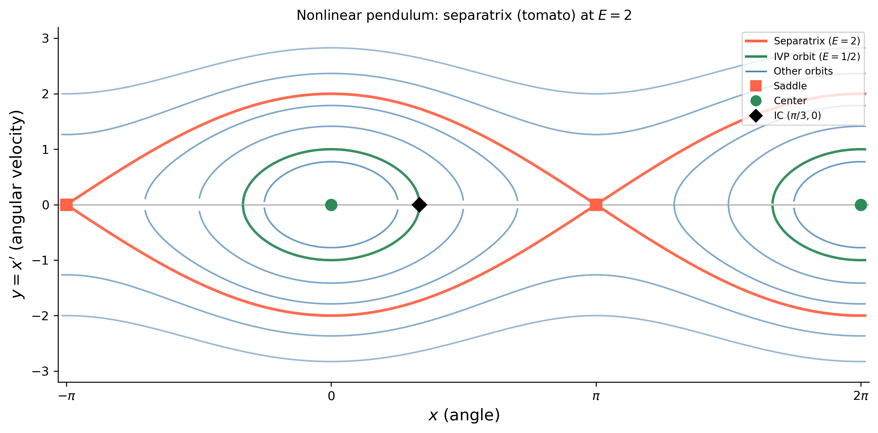
fig, ax = plt.subplots(figsize=(10, 5))
ax.axhline(0, color='gray', lw=0.6)

xr = np.linspace(-np.pi - 0.05, 2*np.pi + 0.05, 1200)
V6_np = 1 - np.cos(xr)

for E_val_np, col, lw, alpha in [
    (2.0,  'tomato',    2.2, 0.95),   # separatrix
    (0.3,  'steelblue', 1.3, 0.8),
    (0.5,  'seagreen',  2.0, 0.95),   # IVP orbit
    (1.0,  'steelblue', 1.3, 0.7),
    (1.6,  'steelblue', 1.3, 0.7),
    (2.8,  'steelblue', 1.3, 0.65),   # rotational orbits
    (4.0,  'steelblue', 1.3, 0.55),
]:
    rhs = 2*(E_val_np - V6_np)
    valid = rhs >= 0
    y_pos =  np.where(valid, np.sqrt(np.maximum(rhs, 0)), np.nan)
    y_neg = -y_pos
    ax.plot(xr, y_pos, color=col, lw=lw, alpha=alpha)
    ax.plot(xr, y_neg, color=col, lw=lw, alpha=alpha)

# Equilibria
for xeq, marker, col, label in [
    (-np.pi, 's', 'tomato',   'Saddle'),
    ( 0,     'o', 'seagreen', 'Center'),
    ( np.pi, 's', 'tomato',   None),
    (2*np.pi,'o', 'seagreen', None),
]:
    ax.plot(xeq, 0, marker, color=col, ms=9, zorder=6,
            label=label if label else '')

# IVP initial condition
ax.plot(np.pi/3, 0, 'D', color='black', ms=8, zorder=7,
        label=r'IC $(\pi/3, 0)$, $E=1/2$')

ax.set_xlim(-np.pi - 0.1, 2*np.pi + 0.1)
ax.set_ylim(-3.2, 3.2)
ax.set_xlabel(r'$x$ (angle)', fontsize=13)
ax.set_ylabel(r"$y = x'$ (angular velocity)", fontsize=13)
ax.set_title('Nonlinear pendulum: separatrix (tomato) at $E=2$', fontsize=11)

# x-axis tick labels at multiples of pi
ax.set_xticks([-np.pi, 0, np.pi, 2*np.pi])
ax.set_xticklabels([r'$-\pi$', r'$0$', r'$\pi$', r'$2\pi$'])

from matplotlib.lines import Line2D
handles = [
    Line2D([0],[0], color='tomato',    lw=2.2, label='Separatrix ($E=2$)'),
    Line2D([0],[0], color='seagreen',  lw=2.0, label=r'IVP orbit ($E=1/2$)'),
    Line2D([0],[0], color='steelblue', lw=1.3, label='Other orbits'),
    Line2D([0],[0], marker='s', color='tomato',  lw=0, ms=8, label='Saddle'),
    Line2D([0],[0], marker='o', color='seagreen',lw=0, ms=8, label='Center'),
    Line2D([0],[0], marker='D', color='black',   lw=0, ms=7,
           label=r'IC $(\pi/3,0)$'),
]
ax.legend(handles=handles, fontsize=8, loc='upper right')
plt.tight_layout()
plt.show()

Figure 6: Phase portrait for Example 6 (nonlinear pendulum \(x''=-\sin x\)). Closed orbits inside the separatrix (tomato) correspond to oscillatory motion; open orbits outside correspond to continuous rotation. The IVP orbit with \(E=1/2\) is highlighted in seagreen, starting at \((\pi/3, 0)\). Saddle points at \(x=\pm\pi\) and centers at \(x=0, 2\pi\) are marked.

---

References

Logan, J David. 2015. A First Course in Differential Equations, Third Edition.

TipExpand for Session Info

import sys
print("Python version:", sys.version)
print('\n'.join(f'{m.__name__}=={m.__version__}'
                for m in globals().values()
                if getattr(m, '__version__', None)))

Python version: 3.14.4 | packaged by conda-forge | (main, Apr  8 2026, 02:33:53) [Clang 20.1.8 ]
numpy==2.4.3
sympy==1.14.0
matplotlib==3.10.8

Reuse

CC BY-NC-SA 4.0