Second-Order Linear Equations — Worked Examples

Show the code
# This is a code cell that imports the necessary libraries for our session.
import numpy as np                        # NumPy for numerical computations
import sympy as sym                       # SymPy for symbolic mathematics
import matplotlib as mpl                  # Matplotlib for plotting
import matplotlib.pyplot as plt           # Matplotlib pyplot interface
from IPython.display import Math, display
mpl.rcParams['figure.dpi'] = 150
mpl.rcParams['axes.spines.top'] = False
mpl.rcParams['axes.spines.right'] = False

In this document we work through fully solved examples for the topics covered in Sections 2.2 and 2.3 of the text:

Each example is worked “by hand” first and then verified using SymPy.


§2.2 Homogeneous Equations

A second-order linear constant-coefficient homogeneous ODE has the form \[ ay'' + by' + cy = 0, \qquad a \neq 0. \] The solution strategy is to substitute the trial function \(y = e^{rt}\) and solve the characteristic equation \[ ar^2 + br + c = 0. \] The nature of the two roots \(r_1, r_2\) determines the form of the general solution.


Example 1 — Real Distinct Roots

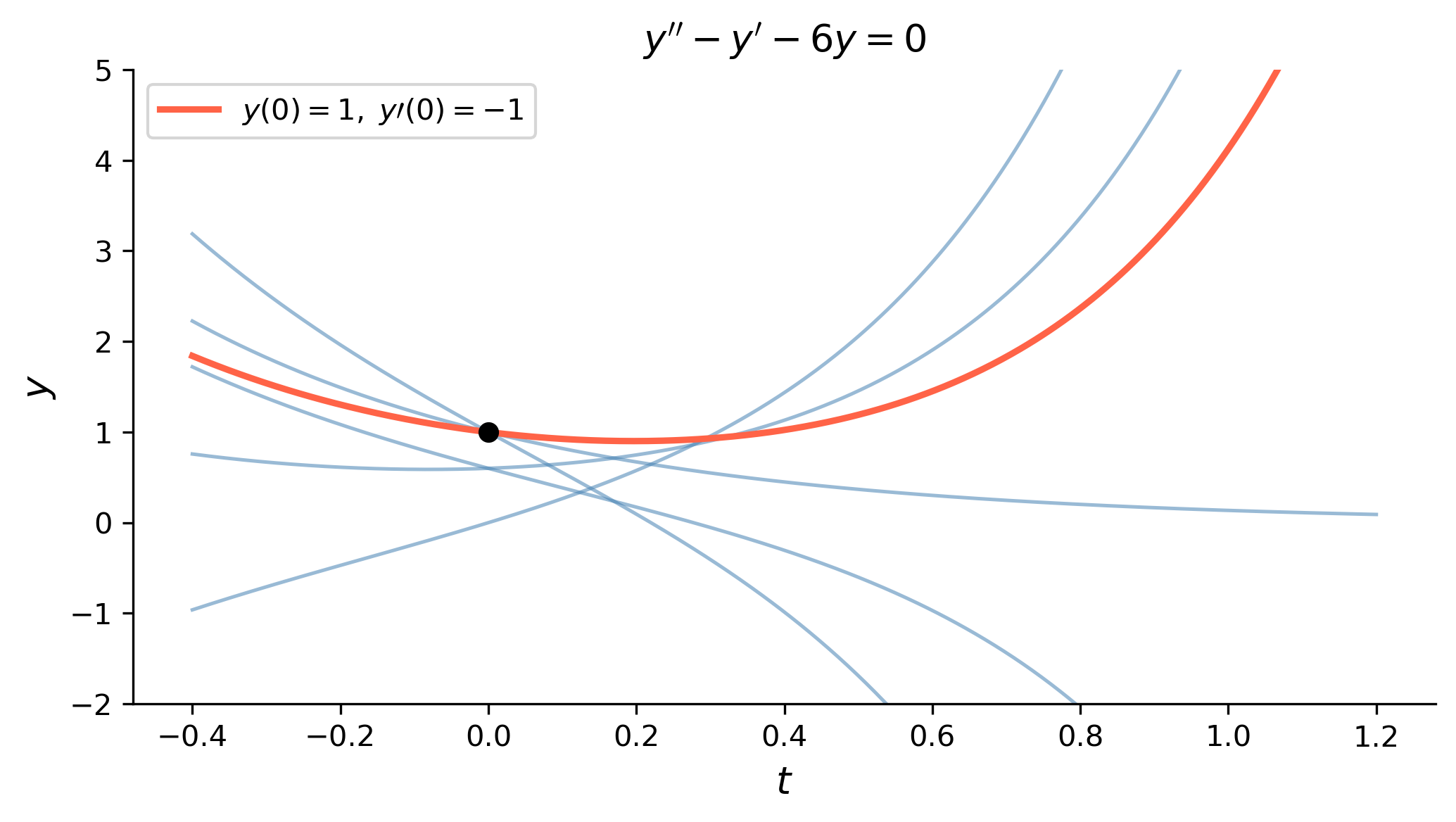
Find the general solution of \[y'' - y' - 6y = 0,\] and solve the initial value problem with \(y(0) = 1\), \(y'(0) = -1\).

By Hand

Step 1 — Write the characteristic equation.

Substituting \(y = e^{rt}\) gives \[ r^2 - r - 6 = 0. \]

Step 2 — Solve for the roots.

Factor: \[ (r - 3)(r + 2) = 0 \quad\Longrightarrow\quad r_1 = 3,\quad r_2 = -2. \]

The roots are real and distinct.

Step 3 — Write the general solution.

Since \(r_1 \neq r_2\) are both real, two linearly independent solutions are \(e^{3t}\) and \(e^{-2t}\), so the general solution is \[ \boxed{y(t) = C_1 e^{3t} + C_2 e^{-2t}.} \]

Step 4 — Apply the initial conditions \(y(0) = 1\), \(y'(0) = -1\).

First differentiate the general solution: \[ y'(t) = 3C_1 e^{3t} - 2C_2 e^{-2t}. \]

Evaluate at \(t = 0\): \[ y(0) = C_1 + C_2 = 1, \] \[ y'(0) = 3C_1 - 2C_2 = -1. \]

Solve the \(2 \times 2\) linear system. From the first equation \(C_1 = 1 - C_2\). Substitute into the second: \[ 3(1 - C_2) - 2C_2 = -1 \;\Longrightarrow\; 3 - 5C_2 = -1 \;\Longrightarrow\; C_2 = \frac{4}{5}. \] Then \(C_1 = 1 - \dfrac{4}{5} = \dfrac{1}{5}\).

The particular solution is \[ \boxed{y(t) = \frac{1}{5}e^{3t} + \frac{4}{5}e^{-2t}.} \]

Tip

Long-run behavior. As \(t \to \infty\) the term \(\tfrac{1}{5}e^{3t}\) dominates since \(3 > -2\), so \(y(t) \to +\infty\). If \(C_1 = 0\) (obtainable by choosing \(y(0) = 0\), \(y'(0) = 2\)), the solution decays to zero.

Using SymPy

t = sym.Symbol('t')
y = sym.Function('y')

ode1 = sym.Eq(y(t).diff(t, 2) - y(t).diff(t) - 6*y(t), 0)

# General solution
gen1 = sym.dsolve(ode1, y(t))
display(Math(r'\text{General solution: }\quad' + sym.latex(gen1)))

# Particular solution with y(0)=1, y'(0)=-1
part1 = sym.dsolve(ode1, y(t), ics={y(0): 1, y(t).diff(t).subs(t, 0): -1})
display(Math(r'\text{Particular solution: }\quad' + sym.latex(part1)))

\(\displaystyle \text{General solution: }\quady{\left(t \right)} = C_{1} e^{- 2 t} + C_{2} e^{3 t}\)

\(\displaystyle \text{Particular solution: }\quady{\left(t \right)} = \frac{e^{3 t}}{5} + \frac{4 e^{- 2 t}}{5}\)

Show the code
t_vals = np.linspace(-0.4, 1.2, 500)
fig, ax = plt.subplots(figsize=(7, 4))

# Several solution curves via different (C1, C2) pairs
for C1, C2 in [(-0.5, 1.5), (0, 1), (0.3, 0.3), (0.5, -0.5), (-0.2, 0.8)]:
    y_sol = C1*np.exp(3*t_vals) + C2*np.exp(-2*t_vals)
    ax.plot(t_vals, y_sol, color='steelblue', lw=1.2, alpha=0.55)

# Particular solution C1=1/5, C2=4/5
y_part = (1/5)*np.exp(3*t_vals) + (4/5)*np.exp(-2*t_vals)
ax.plot(t_vals, y_part, color='tomato', lw=2.2,
        label=r'$y(0)=1,\; y\prime(0)=-1$')
ax.plot(0, 1, 'ko', ms=6, zorder=5)

ax.set_ylim(-2, 5)
ax.set_xlabel(r'$t$', fontsize=13)
ax.set_ylabel(r'$y$', fontsize=13)
ax.set_title(r"$y'' - y' - 6y = 0$", fontsize=13)
ax.legend(fontsize=10)
plt.tight_layout()
plt.show()
Figure 1: Solutions of \(y'' - y' - 6y = 0\) for several initial conditions. The particular solution satisfying \(y(0)=1\), \(y'(0)=-1\) is highlighted in red.

Example 2 — Repeated Root

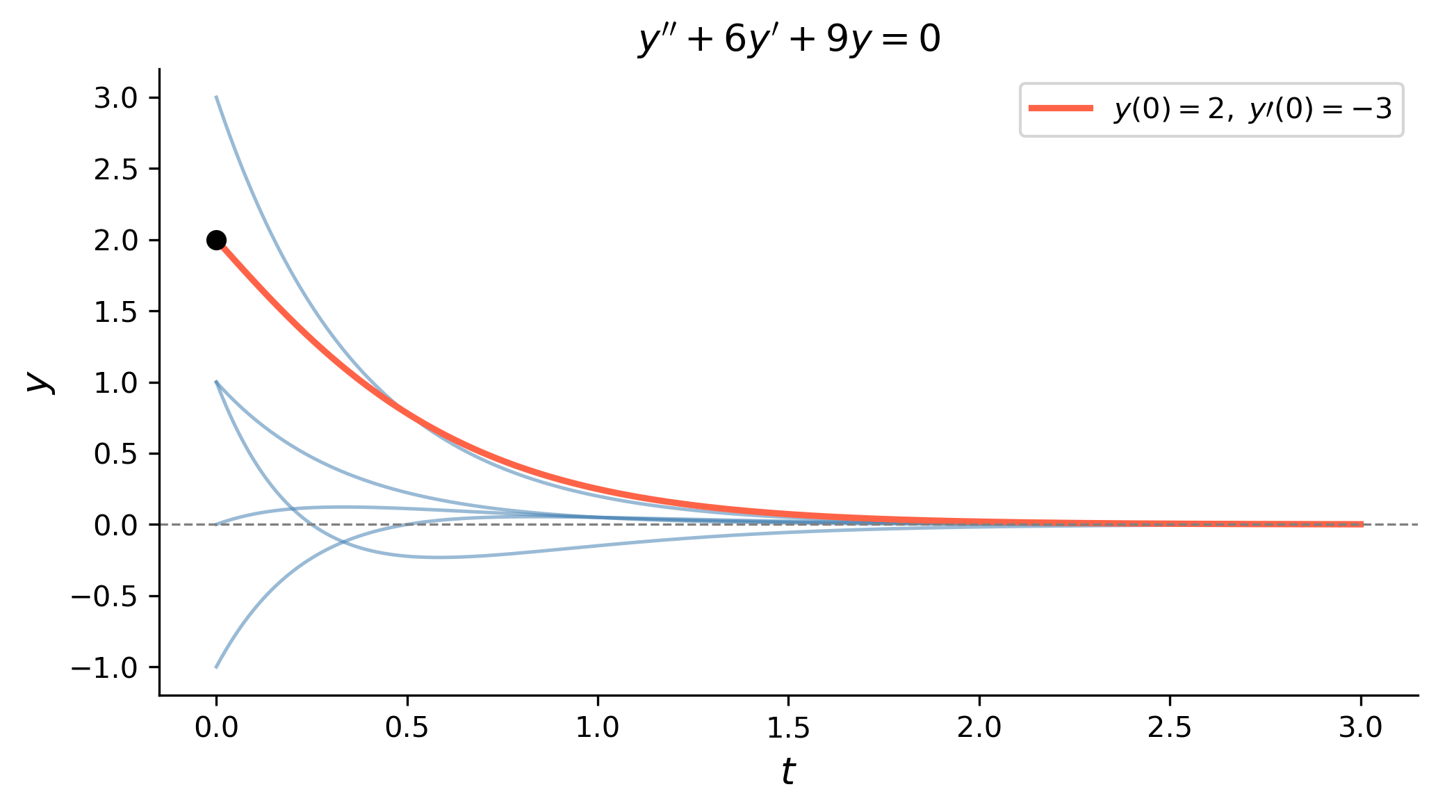
Find the general solution of \[y'' + 6y' + 9y = 0,\] and solve the initial value problem with \(y(0) = 2\), \(y'(0) = -3\).

By Hand

Step 1 — Characteristic equation.

\[ r^2 + 6r + 9 = 0. \]

Step 2 — Solve for the roots.

\[ (r + 3)^2 = 0 \quad\Longrightarrow\quad r = -3 \text{ (repeated root)}. \]

Step 3 — General solution for a repeated root.

When the characteristic equation has a repeated root \(r_1 = r_2 = r\), the two linearly independent solutions are \(e^{rt}\) and \(t e^{rt}\). Here \(r = -3\), so \[ \boxed{y(t) = C_1 e^{-3t} + C_2\, t e^{-3t} = (C_1 + C_2 t)\,e^{-3t}.} \]

Note

Why \(te^{rt}\)? If we only used \(e^{rt}\) twice we would not have two independent solutions. The factor of \(t\) is required to generate a second independent solution; this can be verified rigorously using the method of reduction of order.

Step 4 — Apply the initial conditions \(y(0) = 2\), \(y'(0) = -3\).

Differentiate: \[ y'(t) = -3C_1 e^{-3t} + C_2\bigl(e^{-3t} - 3te^{-3t}\bigr) = (-3C_1 + C_2)e^{-3t} - 3C_2\,te^{-3t}. \]

At \(t = 0\): \[ y(0) = C_1 = 2, \] \[ y'(0) = -3C_1 + C_2 = -3. \]

From the first equation \(C_1 = 2\). Substitute: \[ -3(2) + C_2 = -3 \;\Longrightarrow\; C_2 = -3 + 6 = 3. \]

The particular solution is \[ \boxed{y(t) = (2 + 3t)\,e^{-3t}.} \]

Using SymPy

ode2 = sym.Eq(y(t).diff(t, 2) + 6*y(t).diff(t) + 9*y(t), 0)

gen2 = sym.dsolve(ode2, y(t))
display(Math(r'\text{General solution: }\quad' + sym.latex(gen2)))

part2 = sym.dsolve(ode2, y(t), ics={y(0): 2, y(t).diff(t).subs(t, 0): -3})
display(Math(r'\text{Particular solution: }\quad' + sym.latex(part2)))

\(\displaystyle \text{General solution: }\quady{\left(t \right)} = \left(C_{1} + C_{2} t\right) e^{- 3 t}\)

\(\displaystyle \text{Particular solution: }\quady{\left(t \right)} = \left(3 t + 2\right) e^{- 3 t}\)

Show the code
t_vals = np.linspace(0, 3, 500)
fig, ax = plt.subplots(figsize=(7, 4))

for C1, C2 in [(1, 0), (0, 1), (1, -4), (3, 1), (-1, 2)]:
    y_sol = (C1 + C2*t_vals)*np.exp(-3*t_vals)
    ax.plot(t_vals, y_sol, color='steelblue', lw=1.2, alpha=0.55)

y_part = (2 + 3*t_vals)*np.exp(-3*t_vals)
ax.plot(t_vals, y_part, color='tomato', lw=2.2,
        label=r'$y(0)=2,\; y\prime(0)=-3$')
ax.plot(0, 2, 'ko', ms=6, zorder=5)
ax.axhline(0, color='gray', lw=0.8, ls='--')
ax.set_xlabel(r'$t$', fontsize=13)
ax.set_ylabel(r'$y$', fontsize=13)
ax.set_title(r"$y'' + 6y' + 9y = 0$", fontsize=13)
ax.legend(fontsize=10)
plt.tight_layout()
plt.show()
Figure 2: Solutions of \(y'' + 6y' + 9y = 0\) (repeated root \(r=-3\)). All solutions decay to zero. The particular solution satisfying \(y(0)=2\), \(y'(0)=-3\) is highlighted in red.

Example 3 — Complex Conjugate Roots

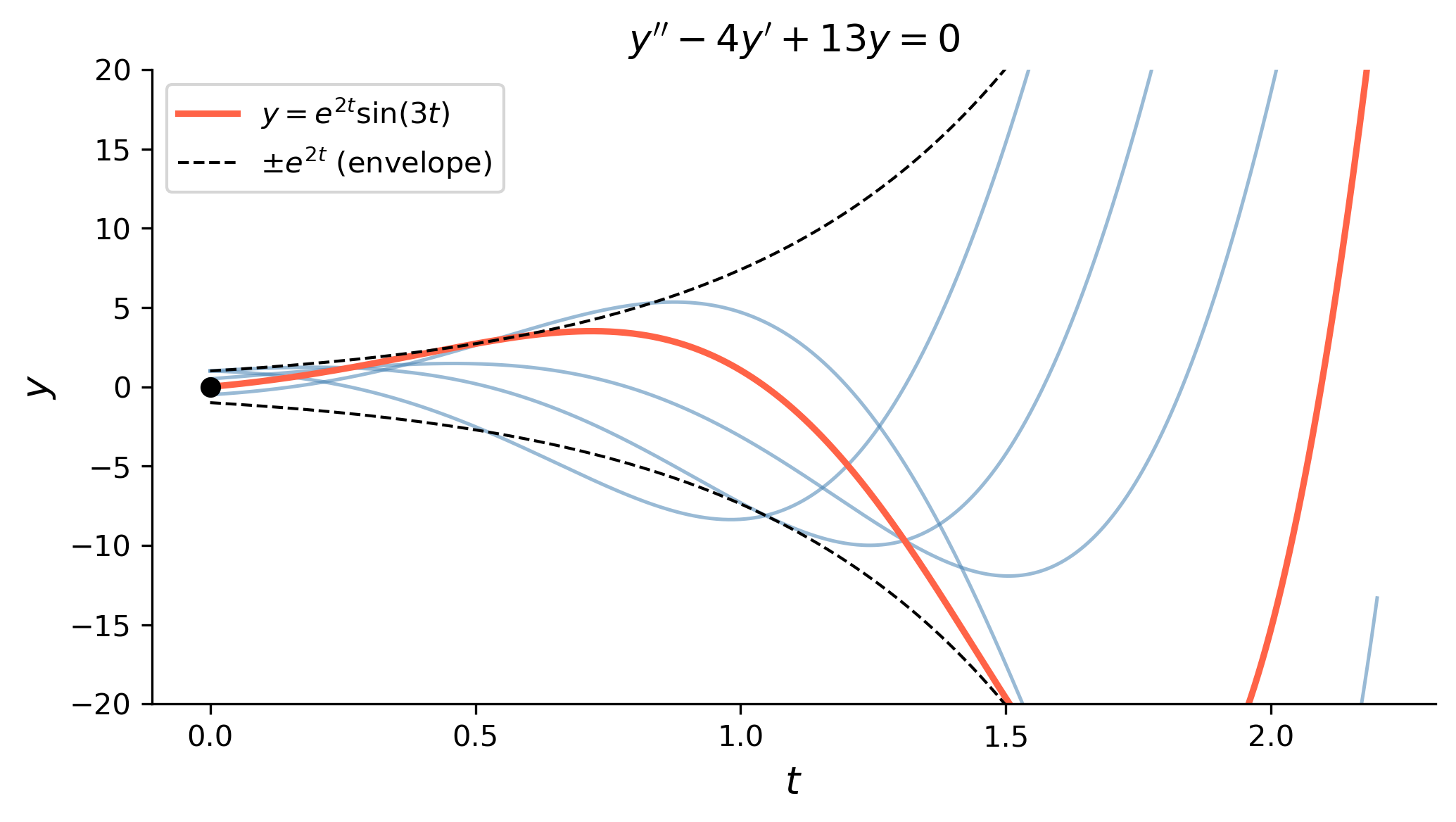
Find the general solution of \[y'' - 4y' + 13y = 0,\] and solve the initial value problem with \(y(0) = 0\), \(y'(0) = 3\).

By Hand

Step 1 — Characteristic equation.

\[ r^2 - 4r + 13 = 0. \]

Step 2 — Solve using the quadratic formula.

\[ r = \frac{4 \pm \sqrt{16 - 52}}{2} = \frac{4 \pm \sqrt{-36}}{2} = \frac{4 \pm 6i}{2} = 2 \pm 3i. \]

The roots are complex conjugates \(r = \alpha \pm \beta i\) with \(\alpha = 2\) and \(\beta = 3\).

Step 3 — Write the general solution.

For complex conjugate roots \(r = \alpha \pm \beta i\), Euler’s formula gives real-valued solutions \(e^{\alpha t}\cos(\beta t)\) and \(e^{\alpha t}\sin(\beta t)\). The general solution is \[ \boxed{y(t) = e^{2t}\bigl[C_1\cos(3t) + C_2\sin(3t)\bigr].} \]

Step 4 — Apply the initial conditions \(y(0) = 0\), \(y'(0) = 3\).

At \(t = 0\): \[ y(0) = e^{0}\bigl[C_1\cos 0 + C_2\sin 0\bigr] = C_1 = 0. \]

Differentiate (using \(C_1 = 0\)): \[ y(t) = C_2 e^{2t}\sin(3t), \] \[ y'(t) = C_2\bigl[2e^{2t}\sin(3t) + 3e^{2t}\cos(3t)\bigr]. \]

At \(t = 0\): \[ y'(0) = C_2\bigl[0 + 3\bigr] = 3C_2 = 3 \;\Longrightarrow\; C_2 = 1. \]

The particular solution is \[ \boxed{y(t) = e^{2t}\sin(3t).} \]

Tip

Amplitude growth. Because \(\alpha = 2 > 0\), the exponential envelope \(e^{2t}\) grows without bound; the oscillations increase in amplitude. If \(\alpha < 0\) the envelope would decay (damped oscillations), and if \(\alpha = 0\) the oscillations would have constant amplitude (pure oscillation).

Using SymPy

ode3 = sym.Eq(y(t).diff(t, 2) - 4*y(t).diff(t) + 13*y(t), 0)

gen3 = sym.dsolve(ode3, y(t))
display(Math(r'\text{General solution: }\quad' + sym.latex(gen3)))

part3 = sym.dsolve(ode3, y(t), ics={y(0): 0, y(t).diff(t).subs(t, 0): 3})
display(Math(r'\text{Particular solution: }\quad' + sym.latex(part3)))

\(\displaystyle \text{General solution: }\quady{\left(t \right)} = \left(C_{1} \sin{\left(3 t \right)} + C_{2} \cos{\left(3 t \right)}\right) e^{2 t}\)

\(\displaystyle \text{Particular solution: }\quady{\left(t \right)} = e^{2 t} \sin{\left(3 t \right)}\)

Show the code
t_vals = np.linspace(0, 2.2, 600)
fig, ax = plt.subplots(figsize=(7, 4))

for C1, C2 in [(1, 0), (0.5, 0.5), (-0.5, 1), (1, -1)]:
    y_sol = np.exp(2*t_vals)*(C1*np.cos(3*t_vals) + C2*np.sin(3*t_vals))
    ax.plot(t_vals, y_sol, color='steelblue', lw=1.2, alpha=0.55)

# Particular solution C1=0, C2=1
y_part = np.exp(2*t_vals)*np.sin(3*t_vals)
ax.plot(t_vals, y_part, color='tomato', lw=2.2,
        label=r'$y = e^{2t}\sin(3t)$')

# Envelope
ax.plot(t_vals,  np.exp(2*t_vals), 'k--', lw=1, label=r'$\pm e^{2t}$ (envelope)')
ax.plot(t_vals, -np.exp(2*t_vals), 'k--', lw=1)
ax.plot(0, 0, 'ko', ms=6, zorder=5)

ax.set_ylim(-20, 20)
ax.set_xlabel(r'$t$', fontsize=13)
ax.set_ylabel(r'$y$', fontsize=13)
ax.set_title(r"$y'' - 4y' + 13y = 0$", fontsize=13)
ax.legend(fontsize=10)
plt.tight_layout()
plt.show()
Figure 3: Solutions of \(y'' - 4y' + 13y = 0\) (complex roots \(r = 2\pm 3i\)). The growing exponential envelope \(\pm e^{2t}\) is shown dashed. The particular solution \(y = e^{2t}\sin(3t)\) is highlighted in red.

§2.3 Nonhomogeneous Equations — Method of Undetermined Coefficients

A nonhomogeneous second-order linear constant-coefficient ODE has the form \[ ay'' + by' + cy = f(t), \] where \(f(t) \not\equiv 0\) is the forcing function. The general solution is \[ y(t) = y_h(t) + y_p(t), \] where \(y_h\) is the general solution of the associated homogeneous equation and \(y_p\) is any particular solution of the full nonhomogeneous equation.

The method of undetermined coefficients finds \(y_p\) by guessing a trial function whose form mirrors that of \(f(t)\), substituting it into the ODE, and matching coefficients. The method applies when \(f(t)\) is a polynomial, an exponential, a sine or cosine, or a product of these.


Example 4 — Polynomial Forcing

Solve the initial value problem \[y'' + 4y' + 4y = 3t^2 - 2, \qquad y(0) = 1,\quad y'(0) = 0.\]

By Hand

Step 1 — Solve the homogeneous equation \(y'' + 4y' + 4y = 0\).

Characteristic equation: \(r^2 + 4r + 4 = (r+2)^2 = 0\), so \(r = -2\) (repeated).

\[ y_h(t) = (C_1 + C_2 t)\,e^{-2t}. \]

Step 2 — Choose a trial particular solution.

Since \(f(t) = 3t^2 - 2\) is a degree-2 polynomial and neither \(t^0\) nor \(t^1\) nor \(t^2\) appears in \(y_h\), we try a full degree-2 polynomial: \[ y_p = At^2 + Bt + D. \] (We use \(D\) instead of \(C\) to avoid confusion with the constants \(C_1\), \(C_2\).)

Step 3 — Compute the required derivatives and substitute.

\[ y_p' = 2At + B, \qquad y_p'' = 2A. \]

Substitute into \(y'' + 4y' + 4y = 3t^2 - 2\): \[ 2A + 4(2At + B) + 4(At^2 + Bt + D) = 3t^2 - 2. \]

Expand and collect by powers of \(t\): \[ 4At^2 + (8A + 4B)t + (2A + 4B + 4D) = 3t^2 - 2. \]

Step 4 — Match coefficients.

Equating coefficients of each power:

Power Equation Result
\(t^2\) \(4A = 3\) \(A = \dfrac{3}{4}\)
\(t^1\) \(8A + 4B = 0\) \(B = -2A = -\dfrac{3}{2}\)
\(t^0\) \(2A + 4B + 4D = -2\) \(4D = -2 - 2\!\left(\tfrac{3}{4}\right) - 4\!\left(-\tfrac{3}{2}\right) = -2 - \tfrac{3}{2} + 6 = \tfrac{5}{2}\), so \(D = \dfrac{5}{8}\)

Thus \[ y_p = \frac{3}{4}t^2 - \frac{3}{2}t + \frac{5}{8}. \]

Step 5 — General solution.

\[ y(t) = (C_1 + C_2 t)\,e^{-2t} + \frac{3}{4}t^2 - \frac{3}{2}t + \frac{5}{8}. \]

Step 6 — Apply the initial conditions.

\[ y(0) = C_1 + \frac{5}{8} = 1 \;\Longrightarrow\; C_1 = \frac{3}{8}. \]

Differentiate: \[ y'(t) = (C_2 - 2C_1 - 2C_2 t)\,e^{-2t} + \frac{3}{2}t - \frac{3}{2}. \]

At \(t = 0\): \[ y'(0) = C_2 - 2C_1 - \frac{3}{2} = 0 \;\Longrightarrow\; C_2 = 2C_1 + \frac{3}{2} = \frac{3}{4} + \frac{3}{2} = \frac{9}{4}. \]

The particular solution is \[ \boxed{y(t) = \left(\frac{3}{8} + \frac{9}{4}t\right)e^{-2t} + \frac{3}{4}t^2 - \frac{3}{2}t + \frac{5}{8}.} \]

Using SymPy

ode4 = sym.Eq(y(t).diff(t, 2) + 4*y(t).diff(t) + 4*y(t), 3*t**2 - 2)

gen4 = sym.dsolve(ode4, y(t))
display(Math(r'\text{General solution: }\quad' + sym.latex(gen4)))

part4 = sym.dsolve(ode4, y(t), ics={y(0): 1, y(t).diff(t).subs(t, 0): 0})
display(Math(r'\text{Particular solution: }\quad' + sym.latex(part4)))

\(\displaystyle \text{General solution: }\quady{\left(t \right)} = \frac{3 t^{2}}{4} - \frac{3 t}{2} + \left(C_{1} + C_{2} t\right) e^{- 2 t} + \frac{5}{8}\)

\(\displaystyle \text{Particular solution: }\quady{\left(t \right)} = \frac{3 t^{2}}{4} - \frac{3 t}{2} + \left(\frac{9 t}{4} + \frac{3}{8}\right) e^{- 2 t} + \frac{5}{8}\)


Example 5 — Exponential Forcing (Standard Case)

Find the general solution of \[y'' - 3y' - 10y = 6e^{2t}.\]

By Hand

Step 1 — Solve the homogeneous equation.

Characteristic equation: \(r^2 - 3r - 10 = (r-5)(r+2) = 0\), giving \(r_1 = 5\), \(r_2 = -2\).

\[ y_h = C_1 e^{5t} + C_2 e^{-2t}. \]

Step 2 — Choose a trial particular solution.

The forcing function is \(f(t) = 6e^{2t}\). Since \(e^{2t}\) does not appear in \(y_h\) (the exponents \(5\) and \(-2\) differ from \(2\)), we try \[ y_p = Ae^{2t}. \]

Step 3 — Substitute and solve for \(A\).

\[ y_p' = 2Ae^{2t}, \qquad y_p'' = 4Ae^{2t}. \]

Substituting into the ODE: \[ 4Ae^{2t} - 3(2Ae^{2t}) - 10(Ae^{2t}) = 6e^{2t} \] \[ (4 - 6 - 10)Ae^{2t} = 6e^{2t} \] \[ -12A = 6 \;\Longrightarrow\; A = -\frac{1}{2}. \]

Step 4 — General solution.

\[ \boxed{y(t) = C_1 e^{5t} + C_2 e^{-2t} - \frac{1}{2}e^{2t}.} \]

Using SymPy

ode5 = sym.Eq(y(t).diff(t, 2) - 3*y(t).diff(t) - 10*y(t), 6*sym.exp(2*t))

gen5 = sym.dsolve(ode5, y(t))
display(Math(r'\text{General solution: }\quad' + sym.latex(gen5)))

\(\displaystyle \text{General solution: }\quady{\left(t \right)} = C_{1} e^{- 2 t} + C_{2} e^{5 t} - \frac{e^{2 t}}{2}\)


Example 6 — Exponential Forcing (Modification Rule)

Find the general solution of \[y'' - 3y' - 10y = 6e^{-2t}.\]

By Hand

Step 1 — Homogeneous solution.

From Example 5 the characteristic roots are \(r_1 = 5\) and \(r_2 = -2\), giving \[ y_h = C_1 e^{5t} + C_2 e^{-2t}. \]

Step 2 — Identify the conflict.

The forcing function \(f(t) = 6e^{-2t}\) has the same exponent \(-2\) as the homogeneous solution \(e^{-2t}\). If we naively tried \(y_p = Ae^{-2t}\), substitution would give \(0 = 6e^{-2t}\) (a contradiction) because \(Ae^{-2t}\) already satisfies the homogeneous equation.

Modification rule: multiply the trial function by \(t\): \[ y_p = Ate^{-2t}. \]

Step 3 — Compute derivatives and substitute.

\[ y_p' = A e^{-2t} - 2At e^{-2t} = A(1 - 2t)e^{-2t}, \] \[ y_p'' = A\bigl[-2e^{-2t} - 2(1-2t)e^{-2t}\bigr] = A(-2 - 2 + 4t)e^{-2t} = A(4t - 4)e^{-2t}. \]

Substitute: \[ A(4t-4)e^{-2t} - 3A(1-2t)e^{-2t} - 10At e^{-2t} = 6e^{-2t}. \]

Factor out \(Ae^{-2t}\) and collect powers of \(t\): \[ A\bigl[(4t - 4) - 3(1 - 2t) - 10t\bigr] = 6. \] \[ A\bigl[4t - 4 - 3 + 6t - 10t\bigr] = 6. \] \[ A\bigl[(4 + 6 - 10)t + (-4 - 3)\bigr] = 6. \] \[ A(0 \cdot t - 7) = 6 \;\Longrightarrow\; A = -\frac{6}{7}. \]

Step 4 — General solution.

\[ \boxed{y(t) = C_1 e^{5t} + C_2 e^{-2t} - \frac{6}{7}\,t e^{-2t}.} \]

Note

Modification rule summary. If the natural trial function for \(y_p\) duplicates a term already present in \(y_h\), multiply the trial by \(t\). If it duplicates a term in \(y_h\) that itself arose from a repeated characteristic root, multiply by \(t^2\).

Using SymPy

ode6 = sym.Eq(y(t).diff(t, 2) - 3*y(t).diff(t) - 10*y(t), 6*sym.exp(-2*t))

gen6 = sym.dsolve(ode6, y(t))
display(Math(r'\text{General solution: }\quad' + sym.latex(gen6)))

\(\displaystyle \text{General solution: }\quady{\left(t \right)} = C_{2} e^{5 t} + \left(C_{1} - \frac{6 t}{7}\right) e^{- 2 t}\)


Example 7 — Sinusoidal Forcing

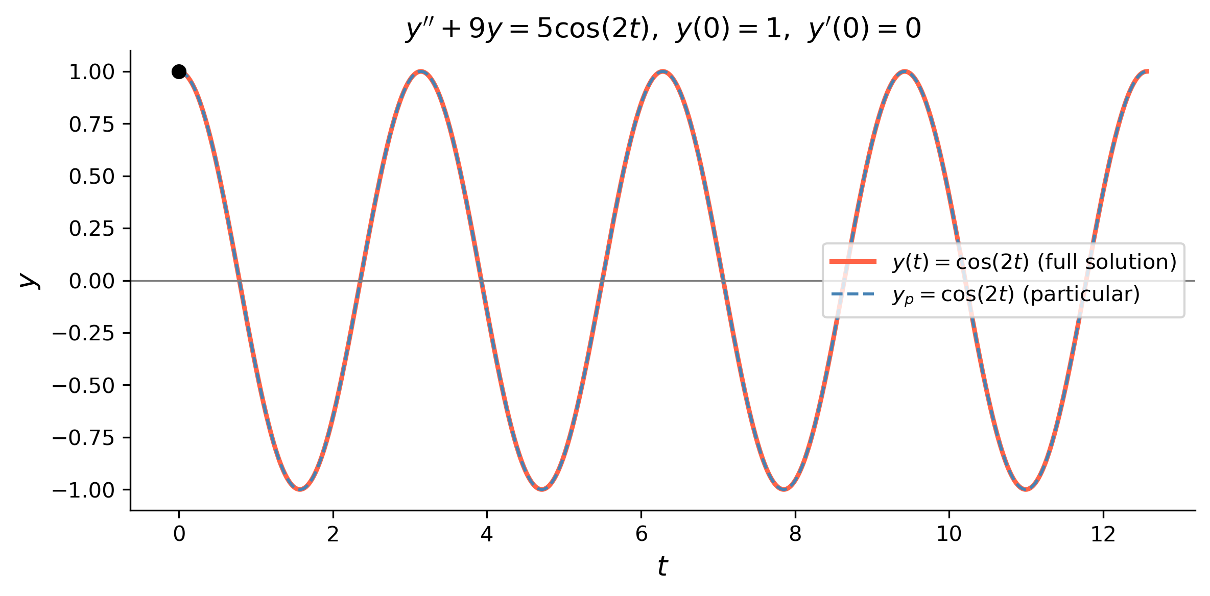
Solve the initial value problem \[y'' + 9y = 5\cos(2t), \qquad y(0) = 1,\quad y'(0) = 0.\]

By Hand

Step 1 — Solve the homogeneous equation \(y'' + 9y = 0\).

Characteristic equation: \(r^2 + 9 = 0 \Rightarrow r = \pm 3i\). So \(\alpha = 0\), \(\beta = 3\): \[ y_h = C_1\cos(3t) + C_2\sin(3t). \]

Step 2 — Choose a trial particular solution.

The forcing function \(f(t) = 5\cos(2t)\) has frequency \(2\), while the homogeneous solutions oscillate at frequency \(3\). Since \(\cos(2t)\) and \(\sin(2t)\) do not appear in \(y_h\) (because \(2 \neq 3\)), we try \[ y_p = A\cos(2t) + B\sin(2t). \]

Step 3 — Substitute.

\[ y_p'' = -4A\cos(2t) - 4B\sin(2t). \]

Substituting into \(y'' + 9y = 5\cos(2t)\): \[ -4A\cos(2t) - 4B\sin(2t) + 9A\cos(2t) + 9B\sin(2t) = 5\cos(2t). \] \[ (9 - 4)A\cos(2t) + (9 - 4)B\sin(2t) = 5\cos(2t). \] \[ 5A\cos(2t) + 5B\sin(2t) = 5\cos(2t). \]

Step 4 — Match coefficients.

\[ 5A = 5 \;\Longrightarrow\; A = 1, \qquad 5B = 0 \;\Longrightarrow\; B = 0. \]

\[ y_p = \cos(2t). \]

Step 5 — General solution.

\[ y(t) = C_1\cos(3t) + C_2\sin(3t) + \cos(2t). \]

Step 6 — Apply the initial conditions.

\[ y(0) = C_1 + 1 = 1 \;\Longrightarrow\; C_1 = 0. \]

Differentiate (using \(C_1 = 0\)): \[ y'(t) = 3C_2\cos(3t) - 2\sin(2t). \] \[ y'(0) = 3C_2 = 0 \;\Longrightarrow\; C_2 = 0. \]

The particular solution is remarkably clean: \[ \boxed{y(t) = \cos(2t).} \]

Tip

This IVP happens to be satisfied by the particular solution alone. In general the homogeneous terms will be nonzero after applying the initial conditions.

Using SymPy

ode7 = sym.Eq(y(t).diff(t, 2) + 9*y(t), 5*sym.cos(2*t))

gen7 = sym.dsolve(ode7, y(t))
display(Math(r'\text{General solution: }\quad' + sym.latex(gen7)))

part7 = sym.dsolve(ode7, y(t), ics={y(0): 1, y(t).diff(t).subs(t, 0): 0})
display(Math(r'\text{Particular solution: }\quad' + sym.latex(part7)))

\(\displaystyle \text{General solution: }\quady{\left(t \right)} = C_{1} \sin{\left(3 t \right)} + C_{2} \cos{\left(3 t \right)} + \cos{\left(2 t \right)}\)

\(\displaystyle \text{Particular solution: }\quady{\left(t \right)} = \cos{\left(2 t \right)}\)

Show the code
t_vals = np.linspace(0, 4*np.pi, 800)

y_full = np.cos(2*t_vals)              # C1 = C2 = 0
y_hom  = np.zeros_like(t_vals)        # homogeneous part vanishes for this IVP
y_part_plot = np.cos(2*t_vals)

fig, ax = plt.subplots(figsize=(8, 4))
ax.plot(t_vals, y_full,      color='tomato',    lw=2.2,
        label=r'$y(t) = \cos(2t)$ (full solution)')
ax.plot(t_vals, y_part_plot, color='steelblue', lw=1.4, ls='--',
        label=r'$y_p = \cos(2t)$ (particular)')
ax.axhline(0, color='gray', lw=0.8)
ax.plot(0, 1, 'ko', ms=6, zorder=5)
ax.set_xlabel(r'$t$', fontsize=13)
ax.set_ylabel(r'$y$', fontsize=13)
ax.set_title(r"$y'' + 9y = 5\cos(2t)$, $\;y(0)=1$, $\;y'(0)=0$", fontsize=13)
ax.legend(fontsize=10)
plt.tight_layout()
plt.show()
Figure 4: Solution of \(y'' + 9y = 5\cos(2t)\) with \(y(0)=1\), \(y'(0)=0\). The particular (forced) response \(\cos(2t)\) and the homogeneous (natural) response are both shown. Here \(C_1 = C_2 = 0\) so the full solution equals the forced response alone.

Example 8 — Sinusoidal Forcing at the Natural Frequency (Resonance)

Find the general solution of \[y'' + 9y = 5\cos(3t).\]

By Hand

Step 1 — Homogeneous solution.

From Example 7, \(y_h = C_1\cos(3t) + C_2\sin(3t)\).

Step 2 — Identify the conflict.

The forcing function \(f(t) = 5\cos(3t)\) oscillates at frequency \(3\), which matches the natural frequency of the system. The trial \(y_p = A\cos(3t) + B\sin(3t)\) would duplicate terms already in \(y_h\).

Modification rule: multiply by \(t\): \[ y_p = At\cos(3t) + Bt\sin(3t). \]

Step 3 — Compute derivatives.

\[ y_p' = A\cos(3t) - 3At\sin(3t) + B\sin(3t) + 3Bt\cos(3t), \] \[ y_p'' = -3A\sin(3t) - 3A\sin(3t) - 9At\cos(3t) + 3B\cos(3t) + 3B\cos(3t) - 9Bt\sin(3t), \] \[ y_p'' = -6A\sin(3t) + 6B\cos(3t) - 9At\cos(3t) - 9Bt\sin(3t). \]

Step 4 — Substitute into \(y'' + 9y = 5\cos(3t)\).

\[ \bigl[-6A\sin(3t) + 6B\cos(3t) - 9At\cos(3t) - 9Bt\sin(3t)\bigr] + 9\bigl[At\cos(3t) + Bt\sin(3t)\bigr] = 5\cos(3t). \]

The \(t\cos\) and \(t\sin\) terms cancel: \[ -6A\sin(3t) + 6B\cos(3t) = 5\cos(3t). \]

Step 5 — Match coefficients.

\[ -6A = 0 \;\Longrightarrow\; A = 0, \qquad 6B = 5 \;\Longrightarrow\; B = \frac{5}{6}. \]

Step 6 — General solution.

\[ \boxed{y(t) = C_1\cos(3t) + C_2\sin(3t) + \frac{5}{6}\,t\sin(3t).} \]

Note

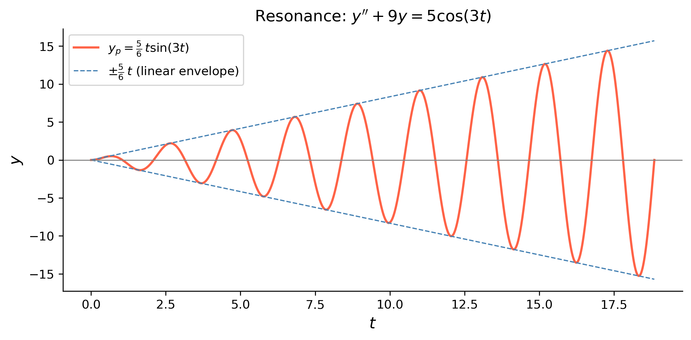
Resonance. The particular solution \(y_p = \dfrac{5}{6}\,t\sin(3t)\) grows in amplitude without bound as \(t \to \infty\) because the forcing frequency exactly matches the system’s natural frequency \(\omega_0 = 3\). This phenomenon is called pure resonance. In physical systems (springs, circuits) even small sustained forces at the natural frequency can produce unbounded oscillations.

Using SymPy

ode8 = sym.Eq(y(t).diff(t, 2) + 9*y(t), 5*sym.cos(3*t))

gen8 = sym.dsolve(ode8, y(t))
display(Math(r'\text{General solution: }\quad' + sym.latex(gen8)))

\(\displaystyle \text{General solution: }\quady{\left(t \right)} = C_{2} \cos{\left(3 t \right)} + \left(C_{1} + \frac{5 t}{6}\right) \sin{\left(3 t \right)}\)

Show the code
t_vals = np.linspace(0, 6*np.pi, 1000)
y_res = (5/6)*t_vals*np.sin(3*t_vals)
envelope = (5/6)*t_vals

fig, ax = plt.subplots(figsize=(8, 4))
ax.plot(t_vals, y_res,      color='tomato',    lw=1.8,
        label=r'$y_p = \frac{5}{6}\,t\sin(3t)$')
ax.plot(t_vals,  envelope,  color='steelblue', lw=1, ls='--',
        label=r'$\pm\frac{5}{6}\,t$ (linear envelope)')
ax.plot(t_vals, -envelope,  color='steelblue', lw=1, ls='--')
ax.axhline(0, color='gray', lw=0.8)
ax.set_xlabel(r'$t$', fontsize=13)
ax.set_ylabel(r'$y$', fontsize=13)
ax.set_title(r"Resonance: $y'' + 9y = 5\cos(3t)$", fontsize=13)
ax.legend(fontsize=10)
plt.tight_layout()
plt.show()
Figure 5: General solution of \(y'' + 9y = 5\cos(3t)\) with \(C_1 = C_2 = 0\), showing the resonant response \(y_p = \tfrac{5}{6}t\sin(3t)\). The amplitude grows linearly with time.

import sys
print("Python version:", sys.version)
print('\n'.join(f'{m.__name__}=={m.__version__}'
                for m in globals().values()
                if getattr(m, '__version__', None)))
Python version: 3.14.4 | packaged by conda-forge | (main, Apr  8 2026, 02:33:53) [Clang 20.1.8 ]
numpy==2.4.3
sympy==1.14.0
matplotlib==3.10.8

Reuse

CC BY-NC-SA 4.0