Variation of Parameters — Worked Examples

Show the code

# This is a code cell that imports the necessary libraries for our session.
import numpy as np                        # NumPy for numerical computations
import sympy as sym                       # SymPy for symbolic mathematics
import matplotlib as mpl                  # Matplotlib for plotting
import matplotlib.pyplot as plt           # Matplotlib pyplot interface
from IPython.display import Math, display
mpl.rcParams['figure.dpi'] = 150
mpl.rcParams['axes.spines.top'] = False
mpl.rcParams['axes.spines.right'] = False

In this document we work through fully solved examples for the topic covered in Section 2.4.2 of the text: the method of variation of parameters for nonhomogeneous second-order linear ODEs.

The examples progress from a gentle warm-up (forcing by a simple exponential) through cases involving rational, trigonometric, and logarithmic forcing functions — precisely the situations where the method of undetermined coefficients does not apply. Each example is worked completely by hand and then verified using SymPy.

The Method — A Brief Review

Consider the nonhomogeneous second-order linear ODE written in standard (divided) form: \[ y'' + p(t)\,y' + q(t)\,y = f(t). \]

Step 0. Solve the associated homogeneous equation \(y'' + p(t)y' + q(t)y = 0\) to obtain two linearly independent solutions \(y_1\) and \(y_2\). The general homogeneous solution is \(y_h = C_1 y_1 + C_2 y_2\).

Step 1 — Form the Wronskian. \[ W(t) = W[y_1, y_2](t) = \begin{vmatrix} y_1 & y_2 \\ y_1' & y_2' \end{vmatrix} = y_1 y_2' - y_2 y_1'. \]

Step 2 — Compute the parameter derivatives. \[ u_1'(t) = -\frac{y_2(t)\,f(t)}{W(t)}, \qquad u_2'(t) = \frac{y_1(t)\,f(t)}{W(t)}. \]

Step 3 — Integrate. \[ u_1(t) = \int u_1'(t)\,dt, \qquad u_2(t) = \int u_2'(t)\,dt. \] (Omit the constants of integration; they fold into \(C_1\) and \(C_2\) of \(y_h\).)

Step 4 — Write the particular solution. \[ y_p(t) = u_1(t)\,y_1(t) + u_2(t)\,y_2(t). \]

Step 5 — General solution. \[ y(t) = y_h(t) + y_p(t) = C_1 y_1 + C_2 y_2 + u_1 y_1 + u_2 y_2. \]

Note

Why variation of parameters? The method of undetermined coefficients is restricted to forcing functions that are polynomials, exponentials, sines, cosines, or products of these. Variation of parameters works for any forcing function \(f(t)\) for which the integrals in Step 3 can be evaluated, including rational functions, \(\sec t\), \(\ln t\), and so on.

Example 1 — Exponential Forcing, Constant-Coefficient ODE

Use the method of variation of parameters to find the general solution of \[y'' - 5y' + 6y = e^t.\]

This example uses a forcing function that could be handled by undetermined coefficients (since \(e^t\) is not a homogeneous solution), but it makes an ideal first example for learning the variation-of-parameters procedure.

By Hand

Step 0 — Homogeneous solution.

Characteristic equation: \(r^2 - 5r + 6 = (r-2)(r-3) = 0\), giving \(r_1 = 2\), \(r_2 = 3\). Thus \[ y_1 = e^{2t}, \quad y_2 = e^{3t}, \quad y_h = C_1 e^{2t} + C_2 e^{3t}. \]

The ODE is already in standard form with \(f(t) = e^t\).

Step 1 — Wronskian. \[ W = y_1 y_2' - y_2 y_1' = e^{2t}\cdot 3e^{3t} - e^{3t}\cdot 2e^{2t} = 3e^{5t} - 2e^{5t} = e^{5t}. \]

Step 2 — Parameter derivatives. \[ u_1' = -\frac{y_2 f}{W} = -\frac{e^{3t} \cdot e^{t}}{e^{5t}} = -\frac{e^{4t}}{e^{5t}} = -e^{-t}, \] \[ u_2' = \frac{y_1 f}{W} = \frac{e^{2t} \cdot e^{t}}{e^{5t}} = \frac{e^{3t}}{e^{5t}} = e^{-2t}. \]

Step 3 — Integrate. \[ u_1 = \int -e^{-t}\,dt = e^{-t}, \qquad u_2 = \int e^{-2t}\,dt = -\frac{1}{2}e^{-2t}. \]

Step 4 — Particular solution. \[ y_p = u_1 y_1 + u_2 y_2 = e^{-t} \cdot e^{2t} + \left(-\frac{1}{2}e^{-2t}\right) e^{3t} = e^{t} - \frac{1}{2}e^{t} = \frac{1}{2}e^{t}. \]

Step 5 — General solution. \[ \boxed{y(t) = C_1 e^{2t} + C_2 e^{3t} + \frac{1}{2}e^{t}.} \]

Tip

Cross-check with undetermined coefficients. Since \(e^t\) is not a solution of the homogeneous equation, we could try \(y_p = Ae^t\). Then \(y_p'' - 5y_p' + 6y_p = Ae^t - 5Ae^t + 6Ae^t = 2Ae^t = e^t\), giving \(A = \tfrac{1}{2}\). This confirms \(y_p = \tfrac{1}{2}e^t\).

Using SymPy

t = sym.Symbol('t')
y = sym.Function('y')

ode1 = sym.Eq(y(t).diff(t, 2) - 5*y(t).diff(t) + 6*y(t), sym.exp(t))

gen1 = sym.dsolve(ode1, y(t))
display(Math(r'\text{General solution: }\quad' + sym.latex(gen1)))

\(\displaystyle \text{General solution: }\quady{\left(t \right)} = \left(C_{1} e^{t} + C_{2} e^{2 t} + \frac{1}{2}\right) e^{t}\)

Example 2 — Rational Forcing: \(\sec t\)

Use variation of parameters to find the general solution of \[y'' + y = \sec t, \qquad -\frac{\pi}{2} < t < \frac{\pi}{2}.\]

The forcing function \(\sec t\) is not of the polynomial-exponential-sinusoidal type, so the method of undetermined coefficients does not apply.

By Hand

Step 0 — Homogeneous solution.

Characteristic equation: \(r^2 + 1 = 0 \Rightarrow r = \pm i\). So \[ y_1 = \cos t, \quad y_2 = \sin t, \quad y_h = C_1\cos t + C_2\sin t. \]

The ODE is already in standard form with \(f(t) = \sec t\).

Step 1 — Wronskian. \[ W = y_1 y_2' - y_2 y_1' = \cos t \cdot \cos t - \sin t \cdot (-\sin t) = \cos^2 t + \sin^2 t = 1. \]

Step 2 — Parameter derivatives. \[ u_1' = -\frac{y_2 f}{W} = -\frac{\sin t \cdot \sec t}{1} = -\frac{\sin t}{\cos t} = -\tan t, \] \[ u_2' = \frac{y_1 f}{W} = \frac{\cos t \cdot \sec t}{1} = \frac{\cos t}{\cos t} = 1. \]

Step 3 — Integrate.

For \(u_1\), recall that \(\displaystyle\int \tan t\,dt = -\ln|\cos t| + C\): \[ u_1 = \int -\tan t\,dt = \ln|\cos t| = \ln(\cos t) \quad\bigl(\text{valid for }|t| < \tfrac{\pi}{2}\bigr). \] \[ u_2 = \int 1\,dt = t. \]

Step 4 — Particular solution. \[ y_p = u_1 y_1 + u_2 y_2 = \ln(\cos t)\cdot\cos t + t\sin t. \]

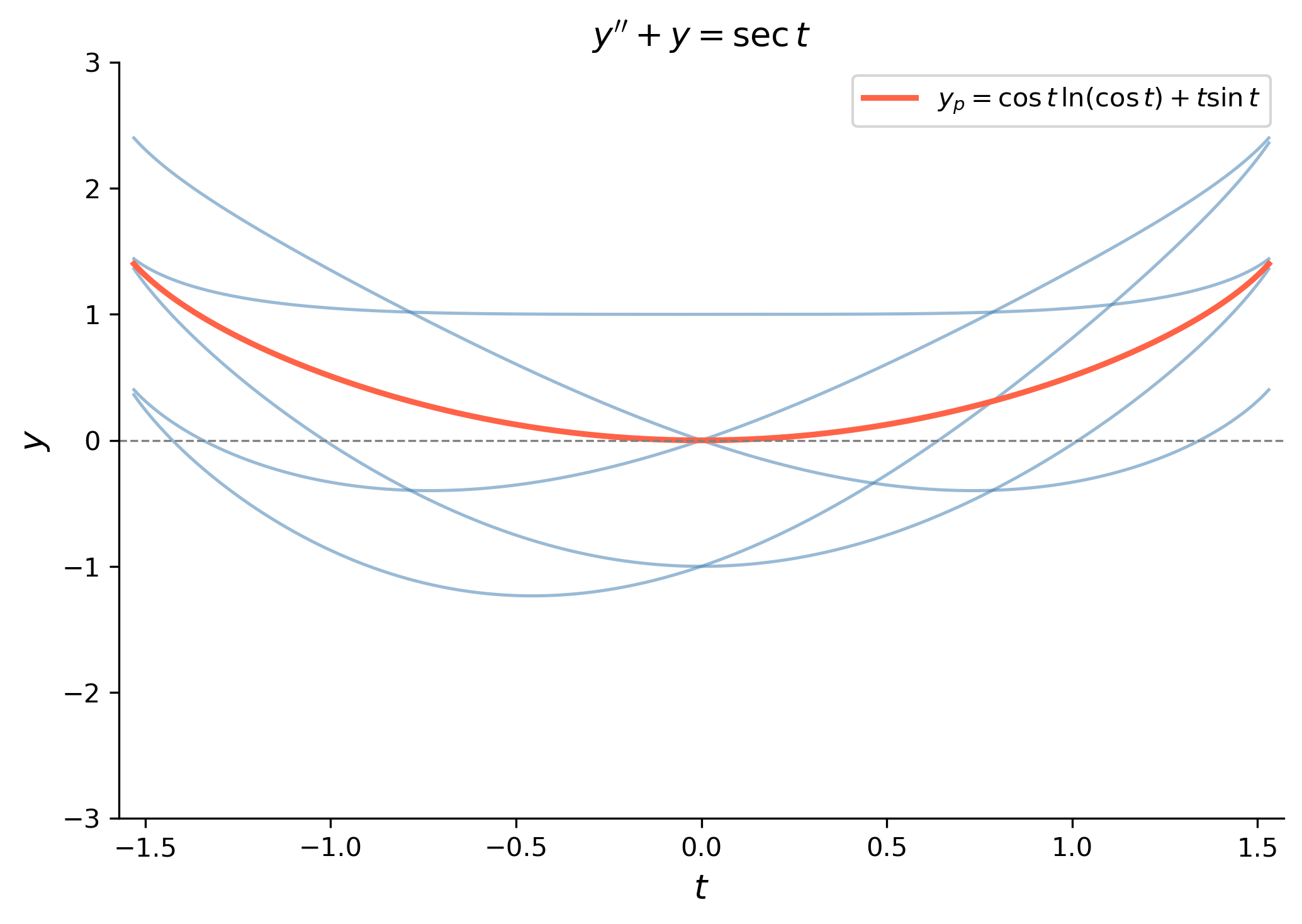
Step 5 — General solution. \[ \boxed{y(t) = C_1\cos t + C_2\sin t + \cos t\,\ln(\cos t) + t\sin t,} \qquad |t| < \frac{\pi}{2}. \]

Note

The term \(\cos t\,\ln(\cos t)\) could never appear as a trial function in the method of undetermined coefficients, which is why variation of parameters is necessary here.

Using SymPy

ode2 = sym.Eq(y(t).diff(t, 2) + y(t), sym.sec(t))

gen2 = sym.dsolve(ode2, y(t))
display(Math(r'\text{General solution: }\quad' + sym.latex(gen2)))

\(\displaystyle \text{General solution: }\quady{\left(t \right)} = \left(C_{1} + t\right) \sin{\left(t \right)} + \left(C_{2} + \log{\left(\cos{\left(t \right)} \right)}\right) \cos{\left(t \right)}\)

Show the code

t_vals = np.linspace(-np.pi/2 + 0.04, np.pi/2 - 0.04, 600)
cos_t  = np.cos(t_vals)
sin_t  = np.sin(t_vals)
yp     = cos_t * np.log(cos_t) + t_vals * sin_t

fig, ax = plt.subplots(figsize=(7, 5))

for C1, C2 in [(-1, 0), (1, 0), (0, -1), (0, 1), (-1, 1)]:
    y_sol = C1*cos_t + C2*sin_t + yp
    ax.plot(t_vals, y_sol, color='steelblue', lw=1.2, alpha=0.55)

ax.plot(t_vals, yp, color='tomato', lw=2.2,
        label=r'$y_p = \cos t\,\ln(\cos t) + t\sin t$')
ax.axhline(0, color='gray', lw=0.8, ls='--')
ax.set_xlim(-np.pi/2, np.pi/2)
ax.set_ylim(-3, 3)
ax.set_xlabel(r'$t$', fontsize=13)
ax.set_ylabel(r'$y$', fontsize=13)
ax.set_title(r"$y'' + y = \sec t$", fontsize=13)
ax.legend(fontsize=10)
plt.tight_layout()
plt.show()

Figure 1: Several solution curves of \(y'' + y = \sec t\) on \((-\pi/2,\,\pi/2)\). The particular solution (red, \(C_1=C_2=0\)) \(y_p = \cos t\ln(\cos t) + t\sin t\) is highlighted.

Example 3 — Rational Forcing: \(1/t^2\)

Use variation of parameters to find the general solution of \[y'' - \frac{2}{t^2}\,y = 3, \qquad t > 0,\] given that \(y_1 = t^2\) and \(y_2 = t^{-1}\) are solutions of the associated homogeneous equation.

Note

This is an Euler–Cauchy type equation (variable coefficients), not a constant-coefficient ODE. Variation of parameters applies to any second-order linear ODE once a fundamental set of solutions is known — the coefficients need not be constant.

By Hand

Step 0 — Homogeneous solution.

We are given \(y_1 = t^2\) and \(y_2 = t^{-1}\). (One may verify by substitution that each satisfies \(y'' - \frac{2}{t^2}y = 0\).)

\[ y_h = C_1 t^2 + C_2 t^{-1}. \]

We must write the ODE in standard form by dividing through by the leading coefficient (here it is already \(1\) for \(y''\)): \[ y'' + 0 \cdot y' - \frac{2}{t^2}\,y = 3. \]

So \(f(t) = 3\).

Step 1 — Wronskian. \[ W = y_1 y_2' - y_2 y_1' = t^2 \cdot \left(-t^{-2}\right) - t^{-1} \cdot 2t = -1 - 2 = -3. \]

Step 2 — Parameter derivatives. \[ u_1' = -\frac{y_2 f}{W} = -\frac{t^{-1} \cdot 3}{-3} = t^{-1}, \] \[ u_2' = \frac{y_1 f}{W} = \frac{t^{2} \cdot 3}{-3} = -t^{2}. \]

Step 3 — Integrate. \[ u_1 = \int t^{-1}\,dt = \ln t, \qquad t > 0, \] \[ u_2 = \int -t^{2}\,dt = -\frac{t^{3}}{3}. \]

Step 4 — Particular solution. \[ y_p = u_1 y_1 + u_2 y_2 = \ln(t) \cdot t^2 + \left(-\frac{t^3}{3}\right) t^{-1} = t^2\ln t - \frac{t^2}{3}. \]

Note

The term \(-\dfrac{t^2}{3}\) is a constant multiple of the homogeneous solution \(y_1 = t^2\) and can be absorbed into \(C_1 t^2\). We therefore simplify the particular solution to \[y_p = t^2 \ln t.\] This is a standard simplification: any part of \(y_p\) that duplicates a homogeneous solution is redundant and may be dropped.

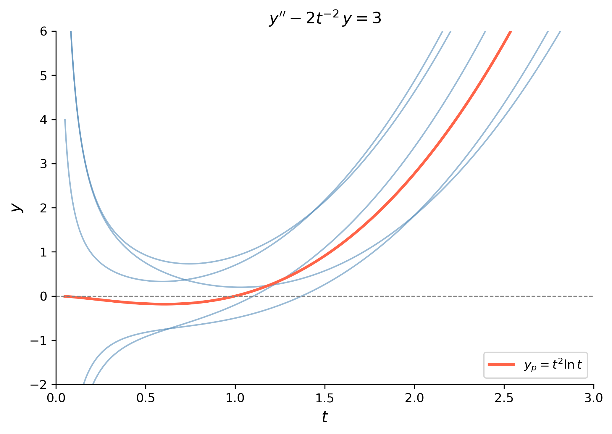
Step 5 — General solution. \[ \boxed{y(t) = C_1 t^2 + C_2 t^{-1} + t^2\ln t, \qquad t > 0.} \]

Verification. Compute \(y_p' = 2t\ln t + t\) and \(y_p'' = 2\ln t + 3\). Then \[ y_p'' - \frac{2}{t^2}y_p = (2\ln t + 3) - \frac{2}{t^2}(t^2\ln t) = 2\ln t + 3 - 2\ln t = 3. \checkmark \]

Using SymPy

Because the coefficient of \(y\) depends on \(t\), we pass the full ODE to dsolve; SymPy recognises it as an Euler–Cauchy equation and handles it symbolically.

ode3 = sym.Eq(y(t).diff(t, 2) - 2/t**2 * y(t), 3)

gen3 = sym.dsolve(ode3, y(t))
display(Math(r'\text{General solution: }\quad' + sym.latex(gen3)))

\(\displaystyle \text{General solution: }\quady{\left(t \right)} = \frac{C_{1} + t^{3} \left(C_{2} + \log{\left(t \right)}\right)}{t}\)

We can also carry out the variation-of-parameters calculation step by step inside SymPy to confirm each stage.

Show the step-by-step SymPy calculation

y1, y2 = t**2, t**(-1)
f3     = sym.Integer(3)

W3 = sym.simplify(y1*sym.diff(y2,t) - y2*sym.diff(y1,t))
display(Math(r'W = ' + sym.latex(W3)))

u1p = sym.simplify(-y2*f3 / W3)
u2p = sym.simplify( y1*f3 / W3)
display(Math(r"u_1' = " + sym.latex(u1p) +
            r",\quad u_2' = " + sym.latex(u2p)))

u1 = sym.integrate(u1p, t)
u2 = sym.integrate(u2p, t)
display(Math(r'u_1 = ' + sym.latex(u1) +
            r',\quad u_2 = ' + sym.latex(u2)))

yp3 = sym.expand(sym.simplify(u1*y1 + u2*y2))
display(Math(r'y_p = ' + sym.latex(yp3)))

\(\displaystyle W = -3\)

\(\displaystyle u_1' = \frac{1}{t},\quad u_2' = - t^{2}\)

\(\displaystyle u_1 = \log{\left(t \right)},\quad u_2 = - \frac{t^{3}}{3}\)

\(\displaystyle y_p = t^{2} \log{\left(t \right)} - \frac{t^{2}}{3}\)

Show the code

t_vals = np.linspace(0.05, 3.0, 500)
yp_vals = t_vals**2 * np.log(t_vals)

fig, ax = plt.subplots(figsize=(7, 5))

for C1, C2 in [(0.5, 0.2), (-0.3, 0.5), (0.2, -0.4), (-0.2, -0.3), (0.4, 0.5)]:
    y_sol = C1*t_vals**2 + C2/t_vals + yp_vals
    ax.plot(t_vals, y_sol, color='steelblue', lw=1.2, alpha=0.55)

ax.plot(t_vals, yp_vals, color='tomato', lw=2.2,
        label=r'$y_p = t^2\ln t$')
ax.axhline(0, color='gray', lw=0.8, ls='--')
ax.set_xlim(0, 3)
ax.set_ylim(-2, 6)
ax.set_xlabel(r'$t$', fontsize=13)
ax.set_ylabel(r'$y$', fontsize=13)
ax.set_title(r"$y'' - 2t^{-2}\,y = 3$", fontsize=13)
ax.legend(fontsize=10)
plt.tight_layout()
plt.show()

Figure 2: Several solution curves of \(y'' - 2t^{-2}y = 3\) for \(t > 0\). The particular solution \(y_p = t^2 \ln t\) (red, \(C_1=C_2=0\)) is highlighted.

Example 4 — Sinusoidal Forcing: \(\csc t\)

Use variation of parameters to find the general solution of \[y'' + 4y = \csc(2t), \qquad 0 < t < \frac{\pi}{2}.\]

By Hand

Step 0 — Homogeneous solution.

Characteristic equation: \(r^2 + 4 = 0 \Rightarrow r = \pm 2i\). So \[ y_1 = \cos(2t), \quad y_2 = \sin(2t), \quad y_h = C_1\cos(2t) + C_2\sin(2t). \]

Standard form: \(f(t) = \csc(2t)\).

Step 1 — Wronskian. \[ W = y_1 y_2' - y_2 y_1' = \cos(2t)\cdot 2\cos(2t) - \sin(2t)\cdot(-2\sin(2t)) = 2\cos^2(2t) + 2\sin^2(2t) = 2. \]

Step 2 — Parameter derivatives. \[ u_1' = -\frac{y_2 f}{W} = -\frac{\sin(2t)\cdot\csc(2t)}{2} = -\frac{1}{2}, \] \[ u_2' = \frac{y_1 f}{W} = \frac{\cos(2t)\cdot\csc(2t)}{2} = \frac{\cos(2t)}{2\sin(2t)} = \frac{1}{2}\cot(2t). \]

Step 3 — Integrate. \[ u_1 = \int -\frac{1}{2}\,dt = -\frac{t}{2}. \]

For \(u_2\), use \(\displaystyle\int \cot(2t)\,dt = \frac{1}{2}\ln|\sin(2t)|\): \[ u_2 = \int \frac{1}{2}\cot(2t)\,dt = \frac{1}{4}\ln|\sin(2t)| = \frac{1}{4}\ln(\sin(2t)) \quad\bigl(0 < t < \tfrac{\pi}{2}\bigr). \]

Step 4 — Particular solution. \[ y_p = u_1 y_1 + u_2 y_2 = \left(-\frac{t}{2}\right)\cos(2t) + \frac{1}{4}\ln(\sin(2t))\cdot\sin(2t). \]

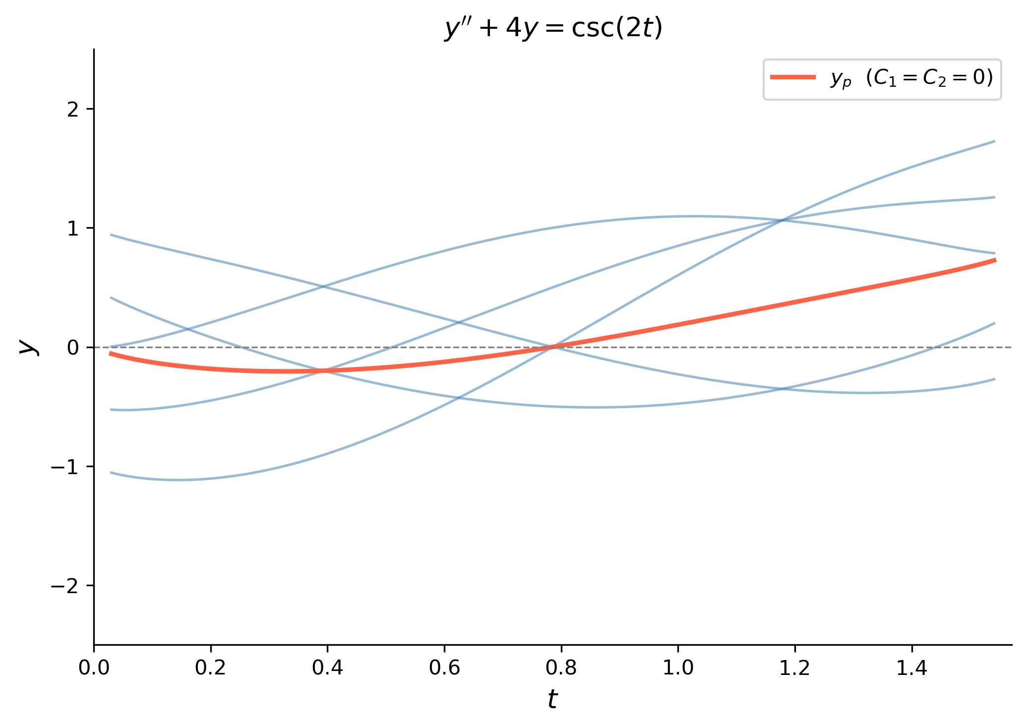
Step 5 — General solution. \[ \boxed{y(t) = C_1\cos(2t) + C_2\sin(2t) - \frac{t}{2}\cos(2t) + \frac{1}{4}\sin(2t)\,\ln(\sin(2t)),} \qquad 0 < t < \frac{\pi}{2}. \]

Using SymPy

ode4 = sym.Eq(y(t).diff(t, 2) + 4*y(t), sym.csc(2*t))

gen4 = sym.dsolve(ode4, y(t))
display(Math(r'\text{General solution: }\quad' + sym.latex(gen4)))

\(\displaystyle \text{General solution: }\quady{\left(t \right)} = \left(C_{1} - \frac{t}{2}\right) \cos{\left(2 t \right)} + \left(C_{2} + \frac{\log{\left(\sin{\left(2 t \right)} \right)}}{4}\right) \sin{\left(2 t \right)}\)

Show the code

t_vals = np.linspace(0.03, np.pi/2 - 0.03, 600)
yp4 = (-t_vals/2)*np.cos(2*t_vals) + (1/4)*np.sin(2*t_vals)*np.log(np.sin(2*t_vals))

fig, ax = plt.subplots(figsize=(7, 5))

for C1, C2 in [(1, 0), (-1, 0), (0, 1), (0.5, -0.5), (-0.5, 0.5)]:
    y_sol = C1*np.cos(2*t_vals) + C2*np.sin(2*t_vals) + yp4
    ax.plot(t_vals, y_sol, color='steelblue', lw=1.2, alpha=0.55)

ax.plot(t_vals, yp4, color='tomato', lw=2.2,
        label=r'$y_p$  ($C_1=C_2=0$)')
ax.axhline(0, color='gray', lw=0.8, ls='--')
ax.set_xlim(0, np.pi/2)
ax.set_ylim(-2.5, 2.5)
ax.set_xlabel(r'$t$', fontsize=13)
ax.set_ylabel(r'$y$', fontsize=13)
ax.set_title(r"$y'' + 4y = \csc(2t)$", fontsize=13)
ax.legend(fontsize=10)
plt.tight_layout()
plt.show()

Figure 3: Several solution curves of \(y'' + 4y = \csc(2t)\) on \((0,\,\pi/2)\). The particular solution (red, \(C_1=C_2=0\)) is highlighted.

Example 5 — An Initial Value Problem

Solve the initial value problem \[y'' - 2y' + y = \frac{e^t}{t^2 + 1}, \qquad y(0) = 0,\quad y'(0) = 1,\qquad t \geq 0.\]

The forcing function \(f(t) = e^t/(t^2+1)\) is not a polynomial-exponential-sinusoidal type, so variation of parameters is required.

By Hand

Step 0 — Homogeneous solution.

Characteristic equation: \(r^2 - 2r + 1 = (r-1)^2 = 0\), so \(r = 1\) is a repeated root. \[ y_1 = e^t, \quad y_2 = te^t, \quad y_h = (C_1 + C_2 t)e^t. \]

Standard form: \(f(t) = \dfrac{e^t}{t^2+1}\).

Step 1 — Wronskian. \[ W = y_1 y_2' - y_2 y_1' = e^t(e^t + te^t) - te^t \cdot e^t = e^{2t} + te^{2t} - te^{2t} = e^{2t}. \]

Step 2 — Parameter derivatives. \[ u_1' = -\frac{y_2 f}{W} = -\frac{te^t \cdot \dfrac{e^t}{t^2+1}}{e^{2t}} = -\frac{t}{t^2+1}, \] \[ u_2' = \frac{y_1 f}{W} = \frac{e^t \cdot \dfrac{e^t}{t^2+1}}{e^{2t}} = \frac{1}{t^2+1}. \]

Step 3 — Integrate.

For \(u_1\), use the substitution \(s = t^2 + 1\), \(ds = 2t\,dt\): \[ u_1 = \int -\frac{t}{t^2+1}\,dt = -\frac{1}{2}\ln(t^2+1). \]

For \(u_2\), recall \(\displaystyle\int \frac{dt}{t^2+1} = \arctan t\): \[ u_2 = \int \frac{dt}{t^2+1} = \arctan t. \]

Step 4 — Particular solution. \[ y_p = u_1 y_1 + u_2 y_2 = \left(-\frac{1}{2}\ln(t^2+1)\right)e^t + (\arctan t)(te^t) = e^t\!\left[t\arctan t - \frac{1}{2}\ln(t^2+1)\right]. \]

Step 5 — General solution. \[ y(t) = (C_1 + C_2 t)e^t + e^t\!\left[t\arctan t - \frac{1}{2}\ln(t^2+1)\right]. \]

Step 6 — Apply the initial conditions.

Evaluate \(y(0) = 0\): \[ y(0) = C_1 e^0 + e^0[0 \cdot \arctan 0 - \tfrac{1}{2}\ln 1] = C_1 = 0 \;\Longrightarrow\; C_1 = 0. \]

Differentiate \(y(t)\) (using \(C_1 = 0\)): \[ y(t) = C_2 t e^t + e^t\!\left[t\arctan t - \frac{1}{2}\ln(t^2+1)\right]. \]

Using the product rule carefully: \[ y'(t) = C_2(e^t + te^t) + e^t\!\left[t\arctan t - \tfrac{1}{2}\ln(t^2+1)\right] + e^t\!\left[\arctan t + \frac{t}{t^2+1} - \frac{t}{t^2+1}\right]. \] \[ y'(t) = C_2(1+t)e^t + e^t\!\left[t\arctan t - \tfrac{1}{2}\ln(t^2+1) + \arctan t\right]. \]

Evaluate \(y'(0) = 1\): \[ y'(0) = C_2(1) + e^0[0 - 0 + \arctan 0] = C_2 = 1 \;\Longrightarrow\; C_2 = 1. \]

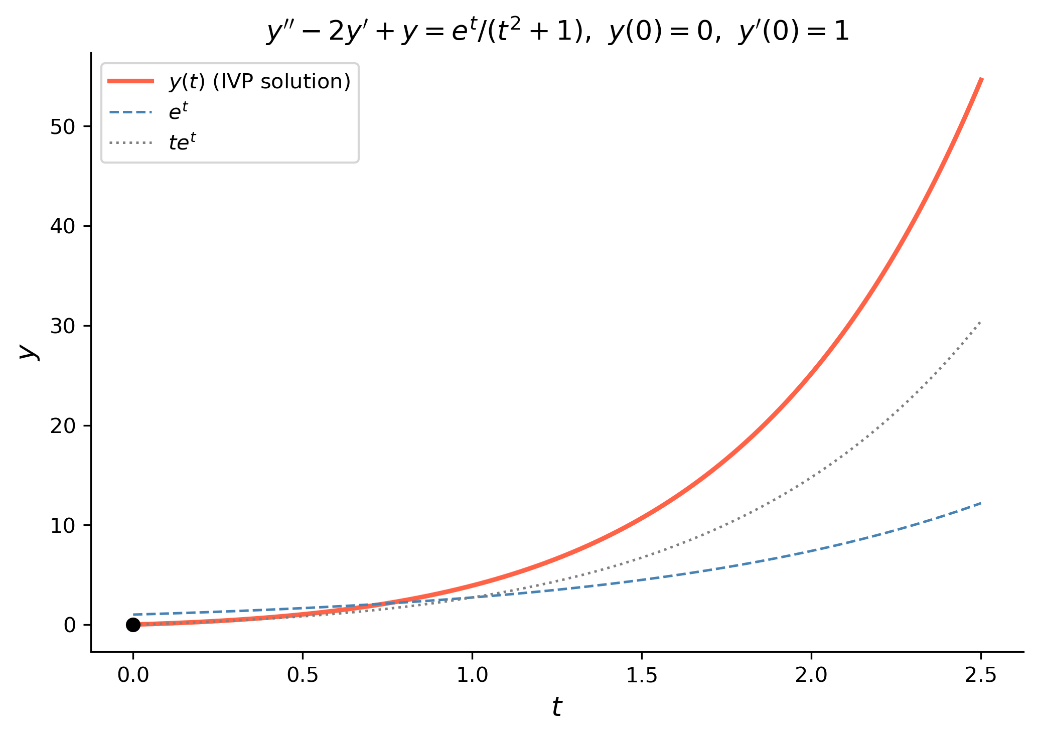
The particular solution to the IVP is \[ \boxed{y(t) = te^t + e^t\!\left[t\arctan t - \frac{1}{2}\ln(t^2+1)\right] = e^t\!\left[t + t\arctan t - \frac{1}{2}\ln(t^2+1)\right].} \]

Using SymPy

SymPy’s dsolve cannot automatically evaluate the variation-of-parameters integrals that produce \(\arctan t\) and \(\ln(t^2+1)\), so we carry out each step of the method explicitly in SymPy instead.

# Homogeneous solutions and forcing function
y1  = sym.exp(t)
y2  = t * sym.exp(t)
f5  = sym.exp(t) / (t**2 + 1)

# Step 1 — Wronskian
W5 = sym.simplify(y1*sym.diff(y2, t) - y2*sym.diff(y1, t))
display(Math(r'W = ' + sym.latex(W5)))

# Step 2 — parameter derivatives
u1p = sym.simplify(-y2 * f5 / W5)
u2p = sym.simplify( y1 * f5 / W5)
display(Math(r"u_1' = " + sym.latex(u1p) +
            r",\quad u_2' = " + sym.latex(u2p)))

# Step 3 — integrate (SymPy handles arctan and log correctly here)
u1 = sym.integrate(u1p, t)
u2 = sym.integrate(u2p, t)
display(Math(r'u_1 = ' + sym.latex(u1)))
display(Math(r'u_2 = ' + sym.latex(u2)))

# Step 4 — particular solution
yp5 = sym.simplify(u1*y1 + u2*y2)
display(Math(r'y_p = ' + sym.latex(yp5)))

\(\displaystyle W = e^{2 t}\)

\(\displaystyle u_1' = - \frac{t}{t^{2} + 1},\quad u_2' = \frac{1}{t^{2} + 1}\)

\(\displaystyle u_1 = - \frac{\log{\left(t^{2} + 1 \right)}}{2}\)

\(\displaystyle u_2 = \operatorname{atan}{\left(t \right)}\)

\(\displaystyle y_p = \left(t \operatorname{atan}{\left(t \right)} - \frac{\log{\left(t^{2} + 1 \right)}}{2}\right) e^{t}\)

# Step 5 — general solution  y = C1*y1 + C2*y2 + yp
C1, C2 = sym.symbols('C1 C2')
y_gen = C1*y1 + C2*y2 + yp5
display(Math(r'y(t) = ' + sym.latex(y_gen)))

\(\displaystyle y(t) = C_{1} e^{t} + C_{2} t e^{t} + \left(t \operatorname{atan}{\left(t \right)} - \frac{\log{\left(t^{2} + 1 \right)}}{2}\right) e^{t}\)

# Step 6 — apply initial conditions y(0)=0, y'(0)=1
ic1 = sym.Eq(y_gen.subs(t, 0), 0)
ic2 = sym.Eq(sym.diff(y_gen, t).subs(t, 0), 1)

consts = sym.solve([ic1, ic2], [C1, C2])
display(Math(r'C_1 = ' + sym.latex(consts[C1]) +
            r',\quad C_2 = ' + sym.latex(consts[C2])))

y_ivp = sym.simplify(y_gen.subs(consts))
display(Math(r'y(t) = ' + sym.latex(y_ivp)))

\(\displaystyle C_1 = 0,\quad C_2 = 1\)

\(\displaystyle y(t) = \left(t \operatorname{atan}{\left(t \right)} + t - \frac{\log{\left(t^{2} + 1 \right)}}{2}\right) e^{t}\)

Verify the IVP solution satisfies the ODE and initial conditions

resid = sym.simplify(
    y_ivp.diff(t, 2) - 2*y_ivp.diff(t) + y_ivp - sym.exp(t)/(t**2 + 1)
)
display(Math(r'\text{ODE residual: }\quad' + sym.latex(resid)))
display(Math(r'y(0) = '  + sym.latex(sym.simplify(y_ivp.subs(t, 0)))))
display(Math(r"y'(0) = " + sym.latex(sym.simplify(y_ivp.diff(t).subs(t, 0)))))

\(\displaystyle \text{ODE residual: }\quad0\)

\(\displaystyle y(0) = 0\)

\(\displaystyle y'(0) = 1\)

Show the code

t_vals   = np.linspace(0, 2.5, 500)
y_ivp_plot = np.exp(t_vals)*(t_vals + t_vals*np.arctan(t_vals)
                             - 0.5*np.log(t_vals**2 + 1))

fig, ax = plt.subplots(figsize=(7, 5))
ax.plot(t_vals, y_ivp_plot,            color='tomato',    lw=2.2,
        label=r'$y(t)$ (IVP solution)')
ax.plot(t_vals, np.exp(t_vals),     color='steelblue', lw=1.2, ls='--',
        label=r'$e^t$')
ax.plot(t_vals, t_vals*np.exp(t_vals), color='gray',   lw=1.2, ls=':',
        label=r'$te^t$')
ax.plot(0, 0, 'ko', ms=6, zorder=5)
ax.set_xlabel(r'$t$', fontsize=13)
ax.set_ylabel(r'$y$', fontsize=13)
ax.set_title(r"$y'' - 2y' + y = e^t/(t^2+1)$, $\;y(0)=0$, $\;y'(0)=1$",
             fontsize=13)
ax.legend(fontsize=10)
plt.tight_layout()
plt.show()

Figure 4: IVP solution \(y(t) = e^t[t + t\arctan t - \tfrac{1}{2}\ln(t^2+1)]\) for \(y'' - 2y' + y = e^t/(t^2+1)\), \(y(0)=0\), \(y'(0)=1\). The homogeneous solutions \(e^t\) (dashed) and \(te^t\) (dotted) are shown for scale.

Summary: When to Use Variation of Parameters vs. Undetermined Coefficients

Situation	Method
\(f(t)\) is a polynomial, \(e^{at}\), \(\sin(bt)\), \(\cos(bt)\), or products/sums of these	Undetermined coefficients (simpler algebra)
\(f(t)\) involves \(\sec t\), \(\csc t\), \(\tan t\), \(\ln t\), \(1/p(t)\), or other non-elementary forms	Variation of parameters (always works when the integrals are tractable)
Variable-coefficient ODE (e.g. Euler–Cauchy) with known \(y_1\), \(y_2\)	Variation of parameters
Either method could work	Undetermined coefficients is usually less labor-intensive

The key formula to memorize is the Wronskian-based pair: \[ u_1' = -\frac{y_2 f}{W}, \qquad u_2' = \frac{y_1 f}{W}, \qquad W = y_1 y_2' - y_2 y_1'. \] Always divide the ODE by the leading coefficient first to put it in standard form before reading off \(f(t)\).

Expand for Session Info

import sys
print("Python version:", sys.version)
print('\n'.join(f'{m.__name__}=={m.__version__}'
                for m in globals().values()
                if getattr(m, '__version__', None)))

Python version: 3.14.4 | packaged by conda-forge | (main, Apr  8 2026, 02:33:53) [Clang 20.1.8 ]
numpy==2.4.3
sympy==1.14.0
matplotlib==3.10.8

Reuse

CC BY-NC-SA 4.0