# This is a code cell that imports the necessary libraries for our session.import numpy as np # NumPy for numerical computationsimport sympy as sym # SymPy for symbolic mathematicsimport matplotlib as mpl # Matplotlib for plottingimport matplotlib.pyplot as plt # Matplotlib pyplot interfacefrom IPython.display import Math, displaympl.rcParams['figure.dpi'] =150mpl.rcParams['axes.spines.top'] =Falsempl.rcParams['axes.spines.right'] =False
In this document we work through fully solved examples for the topics covered in Sections 3.2–3.4 of the text (Logan 2015):
§3.2 — Using Laplace transforms to solve initial value problems, including problems with piecewise (Heaviside) forcing functions and partial-fraction inversion.
§3.3 — The convolution property of the Laplace transform and its use in inverting products of transforms and expressing solutions with arbitrary forcing.
§3.4 — Impulsive (delta-function) forcing — modeling instantaneous kicks, solving IVPs containing \(\delta_a(t)\), and interpreting the impulse response.
Each example is worked “by hand” first and then verified using SymPy.
§3.2 Solving IVPs with Laplace Transforms
The central strategy is:
Take the Laplace transform of both sides of the ODE, using the derivative rule \(\mathcal{L}[x''] = s^2 X - sx(0) - x'(0)\) to incorporate initial conditions algebraically.
Solve the resulting algebraic equation for \(X(s)\).
Invert \(X(s)\) — using partial fractions, the shift theorems, or convolution — to recover \(x(t)\).
Example 1 — Partial Fractions and a Repeated Factor
Solve the initial value problem \[x'' + 4x' + 4x = 8e^{t}, \qquad x(0) = 1,\quad x'(0) = 0.\]
By Hand
Step 1 — Take the Laplace transform.
Let \(X(s) = \mathcal{L}[x(t)]\). Applying the transform and inserting the initial conditions gives \[
\bigl[s^2 X - s(1) - 0\bigr] + 4\bigl[sX - 1\bigr] + 4X = \frac{8}{s - 1}.
\]
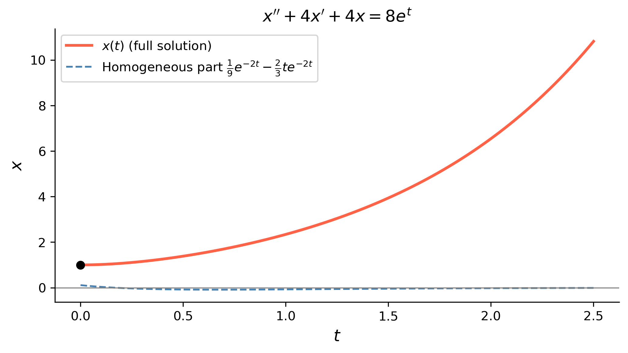
Figure 1: Solution of \(x'' + 4x' + 4x = 8e^t\) with \(x(0)=1\), \(x'(0)=0\). The decaying homogeneous part (dashed) and the growing exponential drive the solution upward for large \(t\).
Example 2 — Piecewise (Heaviside) Forcing
Solve the initial value problem \[x'' + 9x = f(t), \qquad x(0) = 0,\quad x'(0) = 0,\] where the forcing is the rectangular pulse \[f(t) = H(t-1) - H(t-4).\]
By Hand
Step 1 — Laplace transform of \(f(t)\).
By the second shifting theorem, \(\mathcal{L}[H(t-a)] = e^{-as}/s\), so \[
F(s) = \frac{e^{-s} - e^{-4s}}{s}.
\]
Step 2 — Transform the ODE.
With zero initial conditions, \((s^2 + 9)X(s) = F(s)\), giving \[
X(s) = \frac{e^{-s} - e^{-4s}}{s(s^2+9)}.
\]
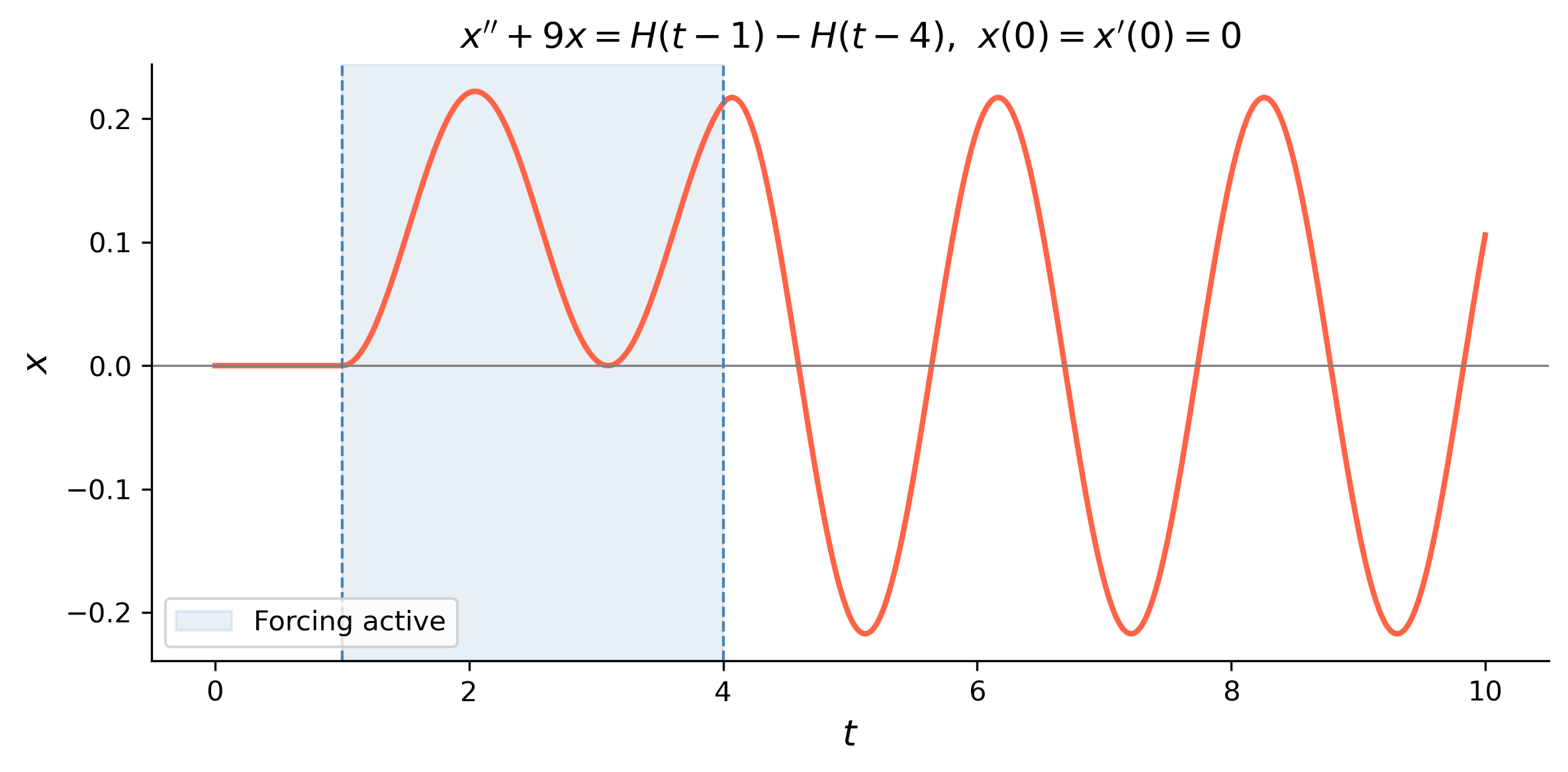
Physical interpretation. The system starts at rest. At \(t=1\) the unit forcing switches on and drives oscillation. At \(t=4\) the forcing switches off; thereafter the system oscillates freely at its natural frequency \(\omega_0 = 3\) with an amplitude determined by the state at \(t=4\).
Figure 2: Response of \(x''+9x=0\) to a rectangular pulse on \([1,4]\). Before \(t=1\) the system is at rest; the pulse drives oscillation, which continues freely after \(t=4\).
Example 3 — Complex Roots and the First Shifting Theorem
Solve the initial value problem \[x'' - 2x' + 5x = 0, \qquad x(0) = 0,\quad x'(0) = 4.\]
Recall \(\mathcal{L}[e^{at}\sin(\omega t)] = \dfrac{\omega}{(s-a)^2 + \omega^2}\). With \(a = 1\) and \(\omega = 2\):
\[
\boxed{x(t) = 2\,e^{t}\sin(2t).}
\]
Tip
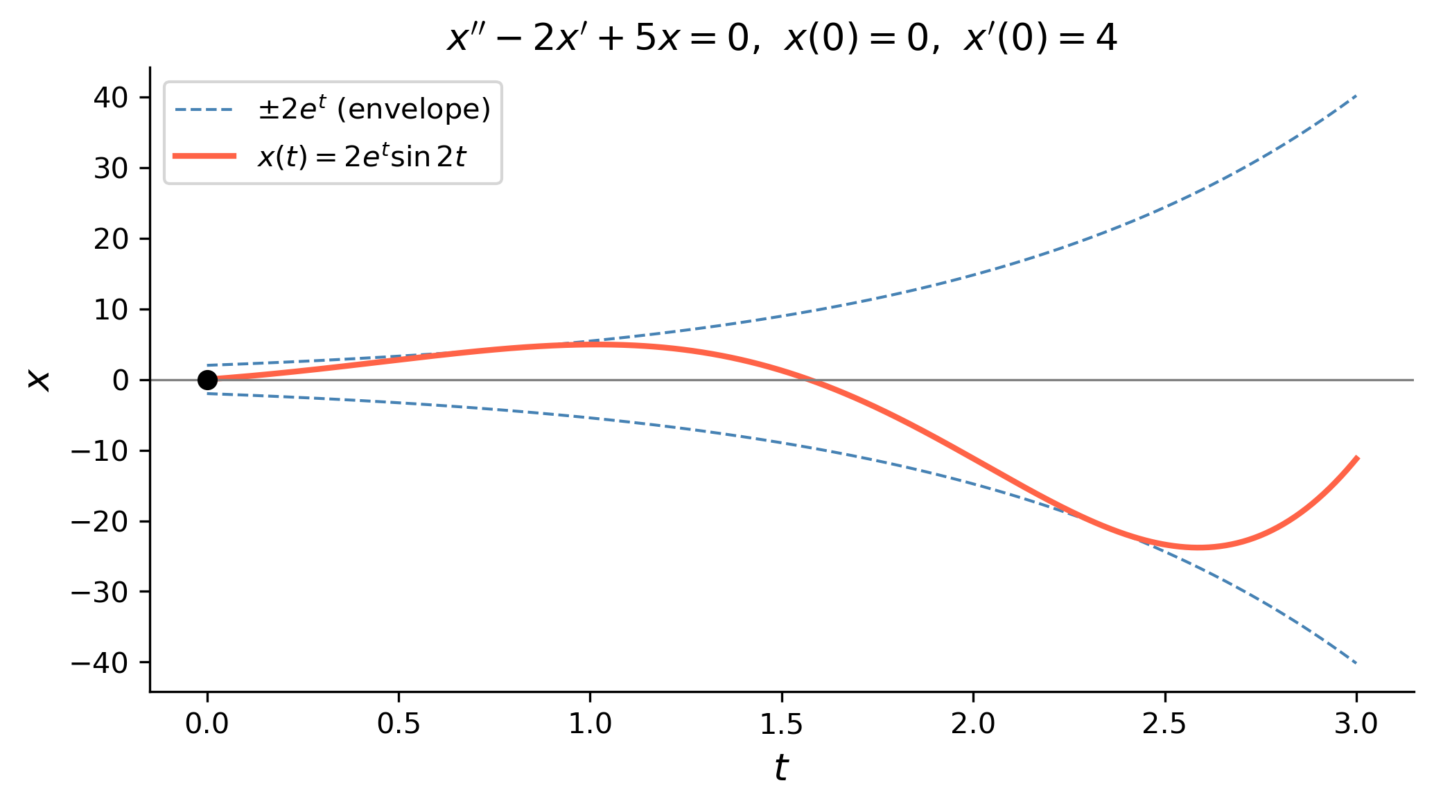
Characteristic equation check. The roots of \(r^2 - 2r + 5 = 0\) are \(r = 1 \pm 2i\). Since \(\alpha = 1 > 0\), the homogeneous solutions grow in amplitude — the system is unstable. This is visible in the plot.
Figure 3: Solution of \(x''-2x'+5x=0\) with \(x(0)=0\), \(x'(0)=4\). The factor \(e^t\) causes the oscillation to grow without bound — the zero equilibrium is unstable.
§3.3 The Convolution Property
If \(\mathcal{L}[f] = F(s)\) and \(\mathcal{L}[g] = G(s)\), then \[
\mathcal{L}^{-1}[F(s)\,G(s)] = (f * g)(t) = \int_0^t f(\tau)\,g(t-\tau)\,d\tau.
\] This is particularly useful when inverting a product \(X(s) = H(s)\,F(s)\), where \(H(s)\) is a system’s transfer function and \(F(s)\) is the transform of the input.
Example 4 — Inverting a Product via Convolution
Use the convolution theorem to compute \[\mathcal{L}^{-1}\!\left[\frac{s}{(s^2+4)^2}\right].\]
Alternative derivation. This result also follows from the transform formula \(\mathcal{L}[t\sin(\omega t)] = \dfrac{2\omega s}{(s^2+\omega^2)^2}\) with \(\omega = 2\): \[
\mathcal{L}\!\left[\frac{t}{4}\sin 2t\right] = \frac{1}{4}\cdot\frac{4s}{(s^2+4)^2}
= \frac{s}{(s^2+4)^2}. \checkmark
\]
Using SymPy
# Verify via inverse Laplace transformexpr4 = s / (s**2+4)**2inv4 = sym.inverse_laplace_transform(expr4, s, t)display(Math(r'\mathcal{L}^{-1}\!\left[\frac{s}{(s^2+4)^2}\right] = '+ sym.latex(sym.simplify(inv4))))# Verify via convolutionf4 = sym.cos(2*t)g4 = sym.sin(2*t) /2conv4 = sym.integrate(f4.subs(t, sym.Symbol('tau'))* g4.subs(t, t - sym.Symbol('tau')), (sym.Symbol('tau'), 0, t))display(Math(r'(f * g)(t) = '+ sym.latex(sym.simplify(conv4))))
\(\displaystyle \mathcal{L}^{-1}\!\left[\frac{s}{(s^2+4)^2}\right] = \frac{t \sin{\left(2 t \right)} \theta\left(t\right)}{4}\)
\(\displaystyle (f * g)(t) = \frac{t \sin{\left(2 t \right)}}{4}\)
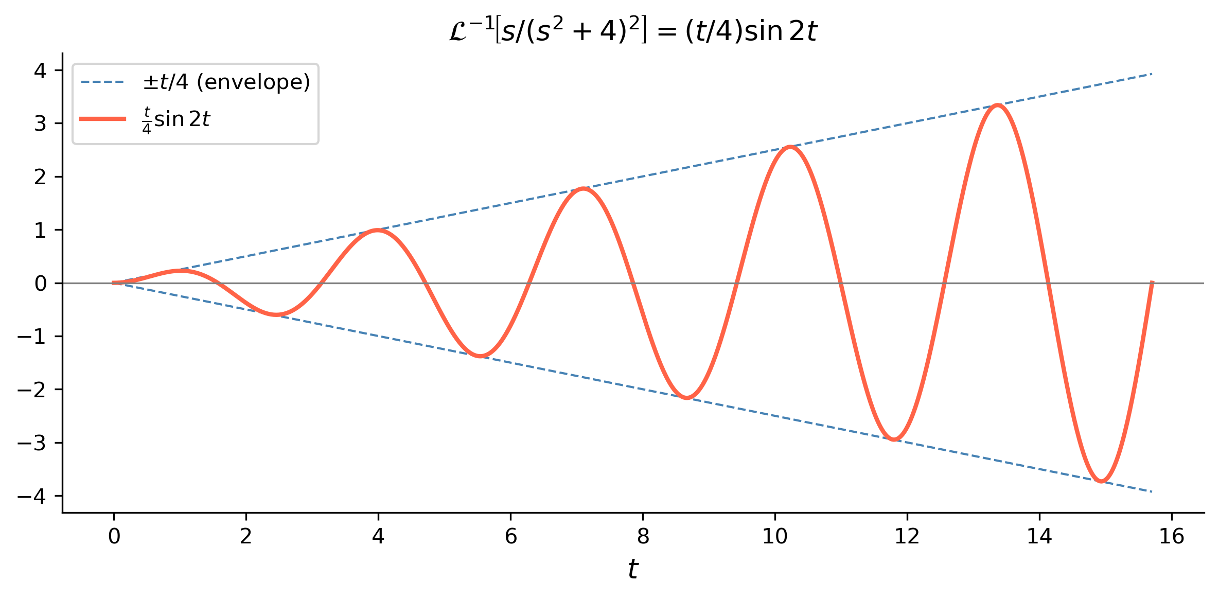
Figure 4: The inverse transform \(x(t)=\tfrac{t}{4}\sin(2t)\). Like the resonance case, the amplitude envelope (dashed) grows linearly — this is the signature of a repeated pole on the imaginary axis.
Example 5 — Solution Formula for an Arbitrary Input
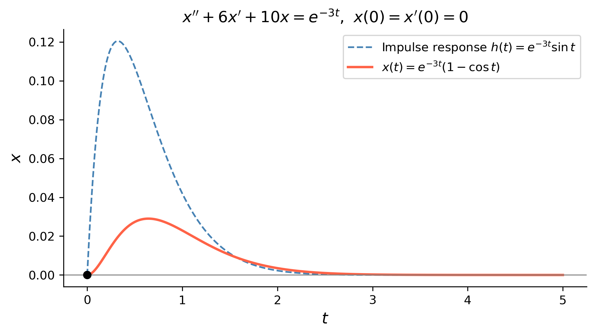
Use the Laplace transform and the convolution property to express the solution of \[x'' + 6x' + 10x = f(t), \qquad x(0) = 0,\quad x'(0) = 0,\] as a convolution integral for any input \(f\). Then evaluate the solution for the specific case \(f(t) = e^{-3t}\).
By Hand
Step 1 — Transform and solve for \(X(s)\).
With zero initial conditions: \[
(s^2 + 6s + 10)\,X(s) = F(s),
\qquad
X(s) = \underbrace{\frac{1}{s^2+6s+10}}_{H(s)}\,F(s).
\]
\(H(s)\) is the transfer function of the system.
Step 2 — Invert the transfer function.
Complete the square: \(s^2+6s+10 = (s+3)^2 + 1\). By the first shifting theorem,
\[
h(t) = \mathcal{L}^{-1}\!\left[\frac{1}{(s+3)^2+1}\right] = e^{-3t}\sin t.
\]
This is the impulse response of the system.
Step 3 — Write the convolution formula.
By the convolution theorem, \[
\boxed{x(t) = (h * f)(t) = \int_0^t e^{-3\tau}\sin\tau\cdot f(t-\tau)\,d\tau.}
\]
Figure 5: Solution of \(x''+6x'+10x = e^{-3t}\) with zero initial conditions. The system is stable (characteristic roots \(-3\pm i\) have negative real part), so the response decays to zero.
Example 6 — Computing a Convolution Directly
Compute the convolution \(f * g\) where \(f(t) = t\) and \(g(t) = e^{2t}\).
For the homogeneous part: \[
\frac{s+2}{(s+2)^2+1} \xrightarrow{\mathcal{L}^{-1}} e^{-2t}\cos t.
\]
For the impulse part, using the second shifting theorem: \[
\frac{e^{-3s}}{(s+2)^2+1} \xrightarrow{\mathcal{L}^{-1}}
e^{-2(t-3)}\sin(t-3)\cdot H(t-3).
\]
Step 4 — Write the full solution.
\[
\boxed{x(t) = e^{-2t}\cos t + e^{-2(t-3)}\sin(t-3)\,H(t-3).}
\]
Note
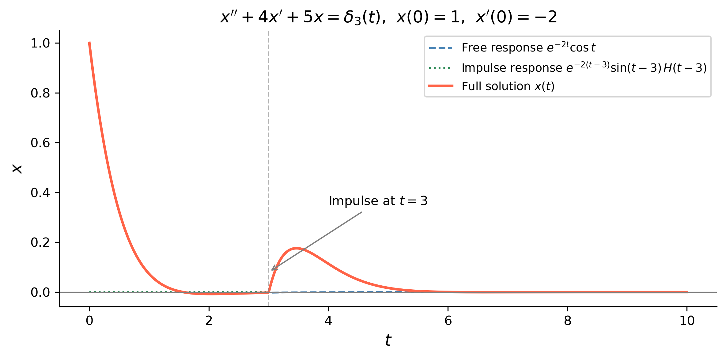
Structure of the solution. For \(0 \le t < 3\), the system evolves freely from the initial conditions: \(x(t) = e^{-2t}\cos t\). At \(t = 3\) the impulse instantaneously adds momentum to the system. For \(t > 3\) the impulse response \(e^{-2(t-3)}\sin(t-3)\) is superimposed on the decaying free response.
Figure 6: Solution of \(x''+4x'+5x=\delta_3(t)\) with \(x(0)=1\), \(x'(0)=-2\). The free response (dashed) decays until the impulse at \(t=3\) kicks the system, adding a new damped oscillation (dotted). The full solution (solid red) is their sum.
Example 8 — Repeated Impulses and Resonance
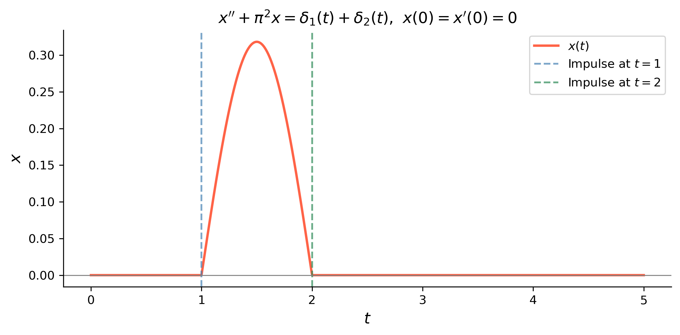
Solve the initial value problem \[x'' + \pi^2 x = \delta_1(t) + \delta_2(t), \qquad x(0) = 0,\quad x'(0) = 0,\] plot the response, and describe what happens physically.
Anti-resonance. Even though each impulse excites oscillation at the natural frequency \(\omega_0 = \pi\), the second impulse arrives exactly one period later and cancels the ongoing oscillation entirely. This is the principle behind vibration cancellation — an impulse timed correctly can null out the response from an earlier impulse.
Figure 7: Response to two impulses at \(t=1\) and \(t=2\). The first impulse excites oscillation at the natural frequency \(\omega_0 = \pi\). The second impulse, arriving exactly one period later, cancels the motion completely for \(t > 2\).
Example 9 — Transfer Function and Impulse Response
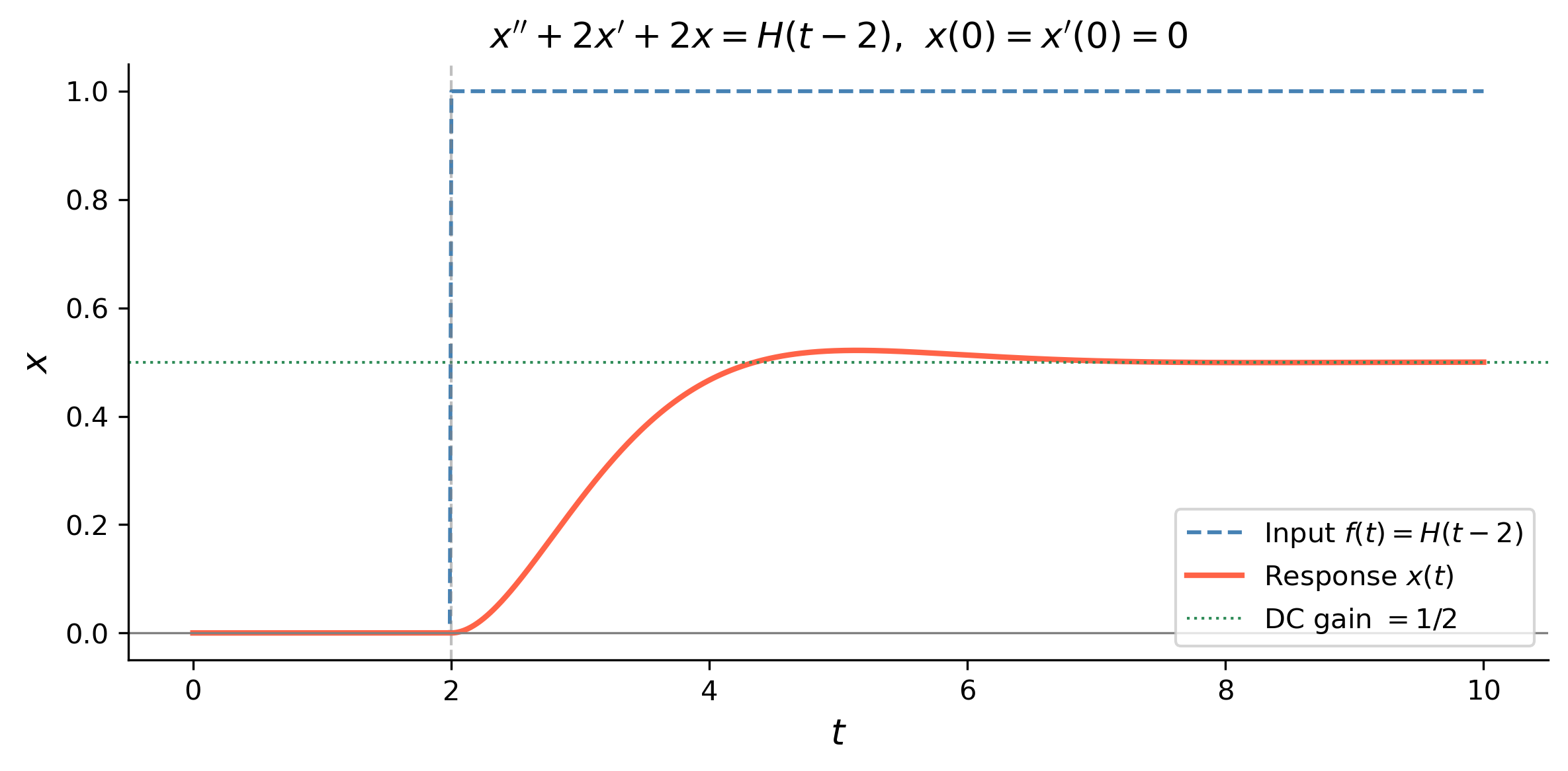
For the system \[x'' + 2x' + 2x = f(t), \qquad x(0) = x'(0) = 0,\](a) find the transfer function \(H(s)\), (b) find the impulse response \(h(t)\), and (c) use convolution to find the response to the input \(f(t) = H(t-2)\) (a unit step switched on at \(t=2\)).
By Hand
Part (a) — Transfer function.
Taking the Laplace transform with zero ICs: \[
(s^2 + 2s + 2)\,X(s) = F(s)
\;\Longrightarrow\;
H(s) = \frac{X(s)}{F(s)} = \frac{1}{s^2+2s+2}.
\]
Part (b) — Impulse response.
Complete the square: \(s^2+2s+2 = (s+1)^2+1\). By the first shifting theorem, \[
h(t) = \mathcal{L}^{-1}\!\left[\frac{1}{(s+1)^2+1}\right] = e^{-t}\sin t.
\]
Part (c) — Step response (delayed step input).
For input \(f(t) = H(t-2)\) we use the convolution formula \(x(t) = (h*f)(t)\).
For \(t < 2\): the Heaviside factor ensures \(f(t-\tau) = H(t-\tau-2) = 0\) when \(\tau > t-2\), and since \(t < 2\) this is zero for all \(\tau \ge 0\), so \(x(t) = 0\).
For \(t \ge 2\): \[
x(t) = \int_0^{t-2} e^{-\tau}\sin\tau\,d\tau.
\]
Using the standard result \(\displaystyle\int e^{-\tau}\sin\tau\,d\tau =
-\tfrac{1}{2}e^{-\tau}(\sin\tau + \cos\tau) + C\):
Combining with the Heaviside factor: \[
\boxed{x(t) = H(t-2)\left\{\frac{1}{2} - \frac{1}{2}e^{-(t-2)}\bigl[\sin(t-2)+\cos(t-2)\bigr]\right\}.}
\]
Note
As \(t\to\infty\) the exponential terms vanish and \(x(t)\to\tfrac{1}{2}\). This is the steady-state response to a unit step, equal to \(H(0) = \tfrac{1}{s^2+2s+2}\big|_{s=0} = \tfrac{1}{2}\) — which is exactly the DC gain of the transfer function.
Figure 8: Response of \(x''+2x'+2x = H(t-2)\) (zero ICs). The delayed step input (dashed) switches on at \(t=2\). The response rises and settles toward the DC gain of \(1/2\) (dotted).
References
Logan, J David. 2015. A First Course in Differential Equations, Third Edition.
TipExpand for Session Info
import sysprint("Python version:", sys.version)print('\n'.join(f'{m.__name__}=={m.__version__}'for m inglobals().values()ifgetattr(m, '__version__', None)))