Phase Plane Analysis and Nonhomogeneous Systems — Worked Examples

Show the code

# This is a code cell that imports the necessary libraries for our session.
import numpy as np                        # NumPy for numerical computations
import sympy as sym                       # SymPy for symbolic mathematics
import matplotlib as mpl                  # Matplotlib for plotting
import matplotlib.pyplot as plt           # Matplotlib pyplot interface
from IPython.display import Math, display
mpl.rcParams['figure.dpi'] = 150
mpl.rcParams['axes.spines.top'] = False
mpl.rcParams['axes.spines.right'] = False

In this document we work through fully solved examples for the topics covered in Sections 4.5 and 4.6 of the text (Logan 2015):

§4.5 — Phase plane analysis of \(\mathbf{x}' = A\mathbf{x}\): sketching phase portraits with nullclines, linear orbits, and direction fields; solving IVPs and plotting solution curves in the phase plane; analyzing systems with a parameter using the trace-determinant plane.
§4.6 — Nonhomogeneous linear systems \(\mathbf{x}' = A\mathbf{x} + \mathbf{f}(t)\): finding equilibria of constant-forced systems, the fundamental matrix, and the variation of parameters formula for particular solutions.

Each example is worked “by hand” first and then verified using NumPy and/or SymPy.

§4.5 Phase Plane Analysis

Given a \(2 \times 2\) linear system \(\mathbf{x}' = A\mathbf{x}\), the nullclines are the curves along which one component of \(\mathbf{x}'\) is zero:

\[ x\text{-nullcline: } x' = 0, \qquad y\text{-nullcline: } y' = 0. \]

For a linear system these are straight lines through the origin. The equilibrium \(\mathbf{x}^* = \mathbf{0}\) lies at their intersection. The type and stability of the origin are read from the trace \(\tau = \operatorname{tr}(A)\) and determinant \(\delta = \det(A)\) via the characteristic equation \(\lambda^2 - \tau\lambda + \delta = 0\):

\[ \lambda = \frac{\tau \pm \sqrt{\tau^2 - 4\delta}}{2}. \]

The trace-determinant plane — with \(\delta\) on the vertical axis and \(\tau\) on the horizontal — organizes all possible phase portrait types: the parabola \(\delta = \tau^2/4\) separates real from complex eigenvalues, the \(\delta\)-axis (\(\tau = 0\)) separates spirals from centers, and the \(\tau\)-axis separates stable from unstable behavior.

Example 1 — Phase Portrait with Nullclines and Two IVP Orbits

A linear system \(\mathbf{x}' = A\mathbf{x}\) has eigenpairs \[ \lambda_1 = -5,\; \mathbf{v}_1 = \begin{pmatrix} 1 \\ 2 \end{pmatrix}; \qquad \lambda_2 = -1,\; \mathbf{v}_2 = \begin{pmatrix} 3 \\ 1 \end{pmatrix}. \] (a) Write the general solution. (b) Identify the critical point type and stability. (c) Find and plot the solution curve satisfying \(\mathbf{x}(0) = (4, 3)^T\), and also the curve satisfying \(\mathbf{x}(0) = (-2, -5)^T\), on the same phase portrait.

By Hand

Step 1 — Recover \(A\) and the nullclines.

Since the eigenpairs are known, we can reconstruct \(A\). The two eigenpairs give \(AP = P\Lambda\) where \(P = [\mathbf{v}_1\;\mathbf{v}_2]\) and \(\Lambda = \operatorname{diag}(\lambda_1,\lambda_2)\), so \(A = P\Lambda P^{-1}\).

\[ P = \begin{pmatrix} 1 & 3 \\ 2 & 1 \end{pmatrix}, \qquad \det P = 1 - 6 = -5, \qquad P^{-1} = \frac{1}{-5}\begin{pmatrix} 1 & -3 \\ -2 & 1 \end{pmatrix}. \]

\[ A = P\Lambda P^{-1} = \begin{pmatrix} 1 & 3 \\ 2 & 1 \end{pmatrix} \begin{pmatrix} -5 & 0 \\ 0 & -1 \end{pmatrix} \frac{1}{-5}\begin{pmatrix} 1 & -3 \\ -2 & 1 \end{pmatrix}. \]

Computing \(P\Lambda\) first:

\[ P\Lambda = \begin{pmatrix} -5 & -3 \\ -10 & -1 \end{pmatrix}. \]

Then \(A = (P\Lambda)P^{-1}\):

\[ A = \frac{1}{-5}\begin{pmatrix} -5 & -3 \\ -10 & -1 \end{pmatrix} \begin{pmatrix} 1 & -3 \\ -2 & 1 \end{pmatrix} = \frac{1}{-5}\begin{pmatrix} -5+6 & 15-3 \\ -10+2 & 30-1 \end{pmatrix} = \frac{1}{-5}\begin{pmatrix} 1 & 12 \\ -8 & 29 \end{pmatrix} = \begin{pmatrix} -\tfrac{1}{5} & -\tfrac{12}{5} \\[4pt] \tfrac{8}{5} & -\tfrac{29}{5} \end{pmatrix}. \]

The \(x\)-nullcline (\(x' = 0\)) is \(-\tfrac{1}{5}x - \tfrac{12}{5}y = 0\), i.e. \(x = -12y\).
The \(y\)-nullcline (\(y' = 0\)) is \(\tfrac{8}{5}x - \tfrac{29}{5}y = 0\), i.e. \(y = \tfrac{8}{29}x\).

Step 2 — General solution.

\[ \boxed{\mathbf{x}(t) = c_1\begin{pmatrix}1\\2\end{pmatrix}e^{-5t} + c_2\begin{pmatrix}3\\1\end{pmatrix}e^{-t}.} \]

In component form: \(x(t) = c_1 e^{-5t} + 3c_2 e^{-t}\), \(\quad y(t) = 2c_1 e^{-5t} + c_2 e^{-t}\).

Step 3 — Classify the critical point.

Both eigenvalues are negative (\(\lambda_1 = -5 < \lambda_2 = -1 < 0\)), so the origin is an asymptotically stable node (sink). The dominant eigenvalue is \(\lambda_2 = -1\) (closer to zero), so all orbits (except those with \(c_2 = 0\)) approach the origin tangent to \(\mathbf{v}_2 = (3,1)^T\).

Step 4 — IVP with \(\mathbf{x}(0) = (4, 3)^T\).

\[ \begin{pmatrix} 1 & 3 \\ 2 & 1 \end{pmatrix} \begin{pmatrix} c_1 \\ c_2 \end{pmatrix} = \begin{pmatrix} 4 \\ 3 \end{pmatrix}. \]

Using \(\det P = -5\):

\[ c_1 = \frac{1}{-5}\det\begin{pmatrix}4&3\\3&1\end{pmatrix} = \frac{4-9}{-5} = \frac{-5}{-5} = 1, \qquad c_2 = \frac{1}{-5}\det\begin{pmatrix}1&4\\2&3\end{pmatrix} = \frac{3-8}{-5} = \frac{-5}{-5} = 1. \]

\[ \mathbf{x}(t) = \begin{pmatrix}1\\2\end{pmatrix}e^{-5t} + \begin{pmatrix}3\\1\end{pmatrix}e^{-t}. \]

Step 5 — IVP with \(\mathbf{x}(0) = (-2, -5)^T\).

\[ \begin{pmatrix} 1 & 3 \\ 2 & 1 \end{pmatrix} \begin{pmatrix} c_1 \\ c_2 \end{pmatrix} = \begin{pmatrix} -2 \\ -5 \end{pmatrix}. \]

\[ c_1 = \frac{(-2)(1)-(3)(-5)}{-5} = \frac{-2+15}{-5} = \frac{13}{-5} = -\frac{13}{5}, \qquad c_2 = \frac{(1)(-5)-(2)(-2)}{-5} = \frac{-5+4}{-5} = \frac{-1}{-5} = \frac{1}{5}. \]

\[ \mathbf{x}(t) = -\frac{13}{5}\begin{pmatrix}1\\2\end{pmatrix}e^{-5t} + \frac{1}{5}\begin{pmatrix}3\\1\end{pmatrix}e^{-t}. \]

Tip

Reading tangency from eigenvalues. Near the origin, the \(c_2 e^{-t}\) term dominates for both IVP orbits (since \(e^{-5t} \to 0\) much faster than \(e^{-t}\)). Both orbits therefore arrive at the origin tangent to the eigenvector direction \((3,1)^T\), confirming the general rule: approach direction is set by the eigenvalue least negative in magnitude.

Using NumPy and SymPy

t = sym.Symbol('t')
c1, c2 = sym.symbols('c1 c2')

v1 = sym.Matrix([1, 2])
v2 = sym.Matrix([3, 1])
lam1, lam2 = -5, -1

# Recover A
P   = sym.Matrix([[1, 3], [2, 1]])
Lam = sym.diag(-5, -1)
A1  = P * Lam * P.inv()
display(Math(r'A = ' + sym.latex(A1)))

# Nullclines
x, y = sym.symbols('x y')
nc_x = sym.solve((A1 * sym.Matrix([x, y]))[0], y)
nc_y = sym.solve((A1 * sym.Matrix([x, y]))[1], y)
display(Math(r'x\text{-nullcline: } y = ' + sym.latex(nc_x[0]) + r'x'))
display(Math(r'y\text{-nullcline: } y = ' + sym.latex(nc_y[0]) + r'x'))

# IVP 1
x0a = sym.Matrix([4, 3])
coeffs_a = P.solve(x0a)
display(Math(r'\mathbf{x}(0)=(4,3)^T:\quad c_1=' + sym.latex(coeffs_a[0])
            + r',\quad c_2=' + sym.latex(coeffs_a[1])))

# IVP 2
x0b = sym.Matrix([-2, -5])
coeffs_b = P.solve(x0b)
display(Math(r'\mathbf{x}(0)=(-2,-5)^T:\quad c_1=' + sym.latex(coeffs_b[0])
            + r',\quad c_2=' + sym.latex(coeffs_b[1])))

\(\displaystyle A = \left[\begin{matrix}- \frac{1}{5} & - \frac{12}{5}\\\frac{8}{5} & - \frac{29}{5}\end{matrix}\right]\)

\(\displaystyle x\text{-nullcline: } y = - \frac{x}{12}x\)

\(\displaystyle y\text{-nullcline: } y = \frac{8 x}{29}x\)

\(\displaystyle \mathbf{x}(0)=(4,3)^T:\quad c_1=1,\quad c_2=1\)

\(\displaystyle \mathbf{x}(0)=(-2,-5)^T:\quad c_1=- \frac{13}{5},\quad c_2=\frac{1}{5}\)

Show the code

v1n = np.array([1, 2], dtype=float)
v2n = np.array([3, 1], dtype=float)
t_f = np.linspace(0,  4, 600)
t_b = np.linspace(0, -1.5, 300)

fig, ax = plt.subplots(figsize=(7, 7))
ax.axhline(0, color='gray', lw=0.6)
ax.axvline(0, color='gray', lw=0.6)

# Background orbits
for c1v, c2v in [(1,0),(-1,0),(0,1),(0,-1),(1,1),(1,-1),(-1,1),(-1,-1),(2,1),(-2,-1)]:
    for tr in [t_f, t_b]:
        xc = c1v*v1n[0]*np.exp(-5*tr) + c2v*v2n[0]*np.exp(-1*tr)
        yc = c1v*v1n[1]*np.exp(-5*tr) + c2v*v2n[1]*np.exp(-1*tr)
        ax.plot(xc, yc, color='gray', lw=0.9, alpha=0.4)

# Nullclines: x-null: x = -12y => y = -x/12; y-null: y = 8x/29
xr = np.linspace(-8, 8, 200)
ax.plot(xr, -xr/12,    color='steelblue', lw=1.6, ls='--', label=r"$x'=0$: $y = -x/12$")
ax.plot(xr,  8*xr/29,  color='darkorange', lw=1.6, ls='--', label=r"$y'=0$: $y = 8x/29$")

# IVP orbit 1: c1=1, c2=1, x(0)=(4,3)
x_a = 1*v1n[0]*np.exp(-5*t_f) + 1*v2n[0]*np.exp(-1*t_f)
y_a = 1*v1n[1]*np.exp(-5*t_f) + 1*v2n[1]*np.exp(-1*t_f)
ax.plot(x_a, y_a, color='tomato', lw=2.2, label=r'IVP: $\mathbf{x}(0)=(4,3)^T$')
ax.plot(4, 3, 'o', color='tomato', ms=7, zorder=5)

# IVP orbit 2: c1=-13/5, c2=1/5, x(0)=(-2,-5)
x_b = (-13/5)*v1n[0]*np.exp(-5*t_f) + (1/5)*v2n[0]*np.exp(-1*t_f)
y_b = (-13/5)*v1n[1]*np.exp(-5*t_f) + (1/5)*v2n[1]*np.exp(-1*t_f)
ax.plot(x_b, y_b, color='seagreen', lw=2.2, label=r'IVP: $\mathbf{x}(0)=(-2,-5)^T$')
ax.plot(-2, -5, 'o', color='seagreen', ms=7, zorder=5)

# Direction arrows on IVP 1
for idx in [60, 140, 240]:
    ax.annotate('', xy=(x_a[idx+6], y_a[idx+6]), xytext=(x_a[idx], y_a[idx]),
                arrowprops=dict(arrowstyle='->', color='tomato', lw=1.4))

ax.plot(0, 0, 'ko', ms=7, zorder=6)
ax.set_xlim(-8, 8)
ax.set_ylim(-7, 7)
ax.set_aspect('equal')
ax.set_xlabel(r'$x$', fontsize=13)
ax.set_ylabel(r'$y$', fontsize=13)
ax.set_title('Stable node with nullclines and two IVP orbits', fontsize=11)
ax.legend(fontsize=9, loc='upper left')
plt.tight_layout()
plt.show()

Figure 1: Phase portrait for Example 1: stable node with \(\lambda_1=-5\), \(\lambda_2=-1\). The \(x\)-nullcline (blue dashed) and \(y\)-nullcline (orange dashed) pass through the origin. Linear orbits along \(\mathbf{v}_1\) (gray) and \(\mathbf{v}_2\) (gray) are shown, with the two IVP solution curves highlighted.

Example 2 — Full Phase Portrait: Repeated Eigenvalue

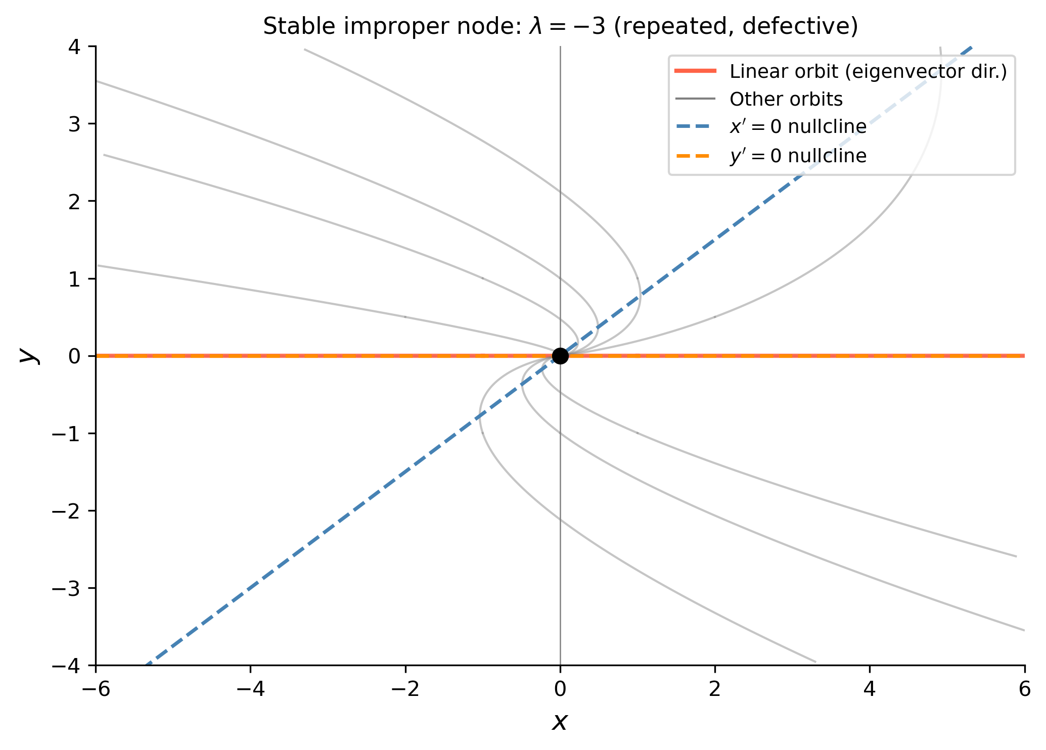
Find the general solution of the system \[ \mathbf{x}' = \begin{pmatrix} -3 & 4 \\ 0 & -3 \end{pmatrix}\mathbf{x}, \] identify the type and stability of the critical point, and sketch the phase portrait including the nullclines.

By Hand

Step 1 — Characteristic equation.

\[ \det(A - \lambda I) = \det\begin{pmatrix}-3-\lambda & 4\\ 0 & -3-\lambda\end{pmatrix} = (-3-\lambda)^2 = 0 \quad\Longrightarrow\quad \lambda = -3 \text{ (repeated)}. \]

Step 2 — Eigenvector.

Solve \((A + 3I)\mathbf{v} = \mathbf{0}\):

\[ \begin{pmatrix} 0 & 4 \\ 0 & 0 \end{pmatrix}\begin{pmatrix}v_1\\v_2\end{pmatrix} = \mathbf{0} \quad\Longrightarrow\quad 4v_2 = 0 \Longrightarrow v_2 = 0,\; v_1 \text{ free}. \]

So \(\mathbf{v} = (1, 0)^T\) is the only (up to scalar) eigenvector. This is a defective matrix (geometric multiplicity 1 < algebraic multiplicity 2).

Step 3 — Generalized eigenvector.

Find \(\mathbf{w}\) satisfying \((A + 3I)\mathbf{w} = \mathbf{v} = (1,0)^T\):

\[ \begin{pmatrix} 0 & 4 \\ 0 & 0 \end{pmatrix}\begin{pmatrix}w_1\\w_2\end{pmatrix} = \begin{pmatrix}1\\0\end{pmatrix} \quad\Longrightarrow\quad 4w_2 = 1 \Longrightarrow w_2 = \frac{1}{4},\; w_1 \text{ free}. \]

Choose \(w_1 = 0\): \(\quad\mathbf{w} = \begin{pmatrix}0 \\ \tfrac{1}{4}\end{pmatrix}\).

Step 4 — Two independent solutions.

For a defective repeated eigenvalue \(\lambda\) with eigenvector \(\mathbf{v}\) and generalized eigenvector \(\mathbf{w}\):

\[ \mathbf{x}_1(t) = \mathbf{v}\,e^{\lambda t}, \qquad \mathbf{x}_2(t) = \bigl(\mathbf{v}\,t + \mathbf{w}\bigr)e^{\lambda t}. \]

Here \(\lambda = -3\):

\[ \mathbf{x}_1(t) = \begin{pmatrix}1\\0\end{pmatrix}e^{-3t}, \qquad \mathbf{x}_2(t) = \left[\begin{pmatrix}1\\0\end{pmatrix}t + \begin{pmatrix}0\\\tfrac{1}{4}\end{pmatrix}\right]e^{-3t} = \begin{pmatrix}t\\\tfrac{1}{4}\end{pmatrix}e^{-3t}. \]

Step 5 — General solution.

\[ \boxed{\mathbf{x}(t) = c_1\begin{pmatrix}1\\0\end{pmatrix}e^{-3t} + c_2\begin{pmatrix}t\\\tfrac{1}{4}\end{pmatrix}e^{-3t}.} \]

In component form: \[ x(t) = (c_1 + c_2 t)\,e^{-3t}, \qquad y(t) = \tfrac{c_2}{4}\,e^{-3t}. \]

Step 6 — Nullclines.

From \(A\mathbf{x} = \mathbf{0}\) with \(A\mathbf{x} \neq \mathbf{0}\):

\(x'\)-nullcline (\(x' = -3x + 4y = 0\)): \(y = \tfrac{3}{4}x\).
\(y'\)-nullcline (\(y' = -3y = 0\)): \(y = 0\) (the \(x\)-axis).

Step 7 — Classification.

The repeated eigenvalue \(\lambda = -3 < 0\) gives an asymptotically stable (improper) node. Because the matrix is defective, all orbits (except the single linear orbit along \(\mathbf{v} = (1,0)^T\)) curve and approach the origin tangent to \(\mathbf{v}\).

Note

Defective node vs. star node. When a repeated eigenvalue has two independent eigenvectors (non-defective, e.g. \(A = \lambda I\)) every direction is an eigenvector and orbits travel in straight lines toward the origin — a star node. When only one eigenvector exists (defective, as here), there is only one linear orbit; all others curve as they enter the origin, forming an improper node.

Using SymPy

A2 = sym.Matrix([[-3, 4], [0, -3]])
lam = sym.Symbol('lambda')

display(Math(r'\text{Eigenvalues: }' + sym.latex(A2.eigenvals())))

for ev, mult, evecs in A2.eigenvects():
    display(Math(r'\lambda=' + sym.latex(ev)
                 + r'\;(\text{mult }' + str(mult) + r'),\quad'
                 + r'\mathbf{v}=' + sym.latex(evecs[0])))

# Generalized eigenvector: (A + 3I)w = v  (singular system, use gauss_jordan_solve)
v_eig = sym.Matrix([1, 0])
# gauss_jordan_solve returns (solution, free_variable_matrix)
w_particular, w_free = (A2 + 3*sym.eye(2)).gauss_jordan_solve(v_eig)
# Set free parameter(s) to zero to get the simplest particular solution
w_gen = w_particular.subs(list(zip(w_free, [0]*len(w_free))))
display(Math(r'\text{Generalized eigenvector: }\mathbf{w}=' + sym.latex(w_gen)))

\(\displaystyle \text{Eigenvalues: }\left\{ -3 : 2\right\}\)

\(\displaystyle \lambda=-3\;(\text{mult }2),\quad\mathbf{v}=\left[\begin{matrix}1\\0\end{matrix}\right]\)

\(\displaystyle \text{Generalized eigenvector: }\mathbf{w}=\left[\begin{matrix}0\\\frac{1}{4}\end{matrix}\right]\)

Show the code

t_f = np.linspace(0,  3.0, 600)
t_b = np.linspace(0, -0.8, 200)

fig, ax = plt.subplots(figsize=(7, 6))
ax.axhline(0, color='gray', lw=0.6)
ax.axvline(0, color='gray', lw=0.6)

# Background orbits: x=(c1+c2*t)*e^{-3t}, y=c2/4*e^{-3t}
for c1v, c2v in [(1,0),(-1,0),(0,4),(0,-4),(1,4),(1,-4),(-1,4),(-1,-4),(2,2),(-2,2)]:
    for tr in [t_f, t_b]:
        xc = (c1v + c2v*tr)*np.exp(-3*tr)
        yc = (c2v/4)*np.exp(-3*tr)
        if c2v == 0:
            ax.plot(xc, yc, color='tomato', lw=2.0, alpha=0.9)
        else:
            mask = (np.abs(xc) < 6) & (np.abs(yc) < 4)
            ax.plot(xc[mask], yc[mask], color='gray', lw=1.0, alpha=0.45)

# Nullclines
xr = np.linspace(-6, 6, 200)
ax.plot(xr, 0.75*xr, color='steelblue', lw=1.7, ls='--', label=r"$x'=0$: $y=\frac{3}{4}x$")
ax.plot(xr, np.zeros_like(xr), color='darkorange', lw=1.7, ls='--', label=r"$y'=0$: $y=0$")

ax.plot(0, 0, 'ko', ms=7, zorder=6)
ax.set_xlim(-6, 6)
ax.set_ylim(-4, 4)
ax.set_aspect('equal')
ax.set_xlabel(r'$x$', fontsize=13)
ax.set_ylabel(r'$y$', fontsize=13)
ax.set_title(r'Stable improper node: $\lambda=-3$ (repeated, defective)', fontsize=11)
from matplotlib.lines import Line2D
handles = [
    Line2D([0],[0], color='tomato',    lw=2, label='Linear orbit (eigenvector dir.)'),
    Line2D([0],[0], color='gray',      lw=1, label='Other orbits'),
    Line2D([0],[0], color='steelblue', lw=1.7, ls='--', label=r"$x'=0$ nullcline"),
    Line2D([0],[0], color='darkorange',lw=1.7, ls='--', label=r"$y'=0$ nullcline"),
]
ax.legend(handles=handles, fontsize=9, loc='upper right')
plt.tight_layout()
plt.show()

Figure 2: Phase portrait for Example 2: asymptotically stable improper node (\(\lambda=-3\) repeated, defective). The single linear orbit along \((1,0)^T\) is shown in tomato; the \(x'\)-nullcline \(y=3x/4\) (steelblue dashed) and \(y'\)-nullcline \(y=0\) (orange dashed) are included.

Example 3 — Bifurcation: Eigenvalue Analysis as a Parameter Varies

Let \(\alpha\) be a real parameter and consider the system \[ \mathbf{x}' = \begin{pmatrix} 2 & -5 \\ \alpha & -2 \end{pmatrix}\mathbf{x}. \] (a) Find the eigenvalues in terms of \(\alpha\). (b) Determine all values of \(\alpha\) at which the type of phase portrait changes and describe the bifurcation. (c) Sketch a representative phase portrait for each qualitatively distinct case.

By Hand

Step 1 — Characteristic equation.

\[ \det(A - \lambda I) = \det\begin{pmatrix}2-\lambda & -5\\ \alpha & -2-\lambda\end{pmatrix} = (2-\lambda)(-2-\lambda) + 5\alpha = \lambda^2 - 4 + 5\alpha = \lambda^2 + (5\alpha - 4). \]

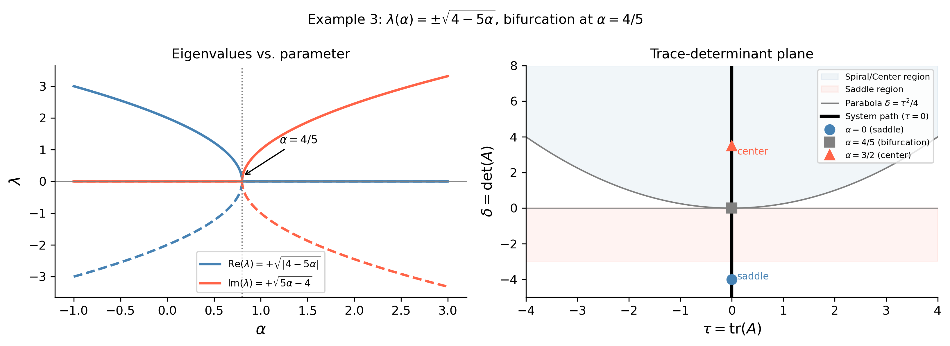
Note: \(\tau = \operatorname{tr}(A) = 0\) for all \(\alpha\), and \(\delta = \det(A) = -4 + 5\alpha\).

So the characteristic equation is \[ \lambda^2 = 4 - 5\alpha \quad\Longrightarrow\quad \lambda = \pm\sqrt{4 - 5\alpha}. \]

Step 2 — Classify by the sign of \(4 - 5\alpha\).

Condition	\(\lambda\)	Phase portrait type	Stability
\(\alpha < \tfrac{4}{5}\)	\(\pm\sqrt{4-5\alpha}\) real, opposite signs	Saddle	Unstable
\(\alpha = \tfrac{4}{5}\)	\(\lambda = 0\) (double)	Non-isolated equilibria	—
\(\tfrac{4}{5} < \alpha\)	\(\pm i\sqrt{5\alpha-4}\) purely imaginary	Center	Stable (not asymptotically)

Step 3 — Bifurcation values.

At \(\alpha = \tfrac{4}{5}\): \(\det(A) = 0\), a line of equilibria appears — the system transitions from a saddle to a center. This is a saddle-to-center bifurcation.
Because \(\tau = 0\) for all \(\alpha\), the eigenvalues are always either real with opposite signs or purely imaginary. There is no spiral behavior for any \(\alpha\).

Step 4 — Representative eigenvalues.

\(\alpha = 0\): \(\lambda = \pm 2\) — saddle.
\(\alpha = \tfrac{4}{5}\): \(\lambda = 0\) — degenerate.
\(\alpha = 1\): \(\lambda = \pm i\) — center (purely imaginary).

\[ \boxed{\lambda(\alpha) = \pm\sqrt{4-5\alpha}.} \]

Tip

Trace-determinant plane. Since \(\tau = 0\) identically, the system’s representative point travels vertically in the trace-determinant plane as \(\alpha\) increases: from the saddle region (\(\delta < 0\), below the \(\tau\)-axis) upward through the bifurcation point \(\delta = 0\) (\(\alpha = 4/5\)) into the center region (\(\delta > 0\), \(\tau = 0\), on the vertical axis above the parabola).

Using SymPy

alpha = sym.Symbol('alpha', real=True)
A3 = sym.Matrix([[2, -5], [alpha, -2]])

tau3   = A3.trace()
delta3 = A3.det()
display(Math(r'\tau = \operatorname{tr}(A) = ' + sym.latex(tau3)))
display(Math(r'\delta = \det(A) = '           + sym.latex(delta3)))

lam_sym = sym.Symbol('lambda')
char3 = A3.charpoly(lam_sym)
roots3 = sym.solve(char3.as_expr(), lam_sym)
display(Math(r'\lambda(\alpha) = ' + sym.latex(roots3)))

bifurc = sym.solve(delta3, alpha)
display(Math(r'\text{Bifurcation at }\alpha = ' + sym.latex(bifurc)))

\(\displaystyle \tau = \operatorname{tr}(A) = 0\)

\(\displaystyle \delta = \det(A) = 5 \alpha - 4\)

\(\displaystyle \lambda(\alpha) = \left[ - \sqrt{4 - 5 \alpha}, \ \sqrt{4 - 5 \alpha}\right]\)

\(\displaystyle \text{Bifurcation at }\alpha = \left[ \frac{4}{5}\right]\)

Show the code

alpha_vals = np.linspace(-1, 3, 800)
disc = 4 - 5*alpha_vals     # = 4 - 5*alpha

# Eigenvalues
lam_real = np.where(disc >= 0,  np.sqrt(np.maximum(disc, 0)), 0.0)
lam_imag = np.where(disc <  0,  np.sqrt(np.maximum(-disc, 0)), 0.0)

fig, axes = plt.subplots(1, 2, figsize=(11, 4))

# Left: eigenvalue vs alpha
ax = axes[0]
ax.plot(alpha_vals,  lam_real, color='steelblue', lw=2, label=r'$\operatorname{Re}(\lambda)=+\sqrt{|4-5\alpha|}$')
ax.plot(alpha_vals, -lam_real, color='steelblue', lw=2, ls='--')
ax.plot(alpha_vals,  lam_imag, color='tomato',    lw=2, label=r'$\operatorname{Im}(\lambda)=+\sqrt{5\alpha-4}$')
ax.plot(alpha_vals, -lam_imag, color='tomato',    lw=2, ls='--')
ax.axvline(4/5, color='gray', lw=1.0, ls=':')
ax.axhline(0,   color='gray', lw=0.6)
ax.annotate(r'$\alpha=4/5$', xy=(4/5, 0.15), xytext=(1.2, 1.2),
            arrowprops=dict(arrowstyle='->', color='black'), fontsize=9)
ax.set_xlabel(r'$\alpha$', fontsize=13)
ax.set_ylabel(r'$\lambda$', fontsize=13)
ax.set_title('Eigenvalues vs. parameter', fontsize=11)
ax.legend(fontsize=8)

# Right: trace-determinant plane
tau_path   = np.zeros_like(alpha_vals)          # always 0
delta_path = -4 + 5*alpha_vals

tau_range  = np.linspace(-4, 4, 400)
parab = tau_range**2 / 4

ax = axes[1]
ax.fill_between(tau_range, parab, 8, alpha=0.07, color='steelblue', label='Spiral/Center region')
ax.fill_between(tau_range, -3, 0, alpha=0.07, color='tomato', label='Saddle region')
ax.plot(tau_range, parab, color='gray', lw=1.2, label='Parabola $\\delta=\\tau^2/4$')
ax.axhline(0, color='gray', lw=0.8)
ax.axvline(0, color='gray', lw=0.8)

# Path of the system
ax.plot(tau_path, delta_path, color='black', lw=2.5, label='System path ($\\tau=0$)')
# Mark key points
ax.plot(0, -4 + 5*0,   'o', color='steelblue', ms=8, label=r'$\alpha=0$ (saddle)')
ax.plot(0, -4 + 5*0.8, 's', color='gray',      ms=8, label=r'$\alpha=4/5$ (bifurcation)')
ax.plot(0, -4 + 5*1.5, '^', color='tomato',    ms=8, label=r'$\alpha=3/2$ (center)')

ax.annotate(r'saddle', xy=(0.1, -4), fontsize=8, color='steelblue')
ax.annotate(r'center', xy=(0.1,  3), fontsize=8, color='tomato')

ax.set_xlim(-4, 4)
ax.set_ylim(-5, 8)
ax.set_xlabel(r'$\tau = \operatorname{tr}(A)$', fontsize=12)
ax.set_ylabel(r'$\delta = \det(A)$', fontsize=12)
ax.set_title('Trace-determinant plane', fontsize=11)
ax.legend(fontsize=7, loc='upper right')

plt.suptitle(r'Example 3: $\lambda(\alpha)=\pm\sqrt{4-5\alpha}$, bifurcation at $\alpha=4/5$',
             fontsize=11)
plt.tight_layout()
plt.show()

Figure 3: Left: real and imaginary parts of the eigenvalues \(\lambda(\alpha)=\pm\sqrt{4-5\alpha}\) vs. \(\alpha\). Right: path traced in the trace-determinant plane as \(\alpha\) increases from \(-1\) to \(3\); the system crosses from saddle (below the \(\tau\)-axis) to center (on the vertical axis, above the parabola) at \(\alpha=4/5\).

§4.6 Nonhomogeneous Systems

A nonhomogeneous linear system has the form

\[ \mathbf{x}' = A\mathbf{x} + \mathbf{f}(t). \]

The general solution is \(\mathbf{x}(t) = \mathbf{x}_h(t) + \mathbf{x}_p(t)\), where \(\mathbf{x}_h = c_1\mathbf{x}_1 + c_2\mathbf{x}_2\) is the general homogeneous solution and \(\mathbf{x}_p\) is any particular solution.

The fundamental matrix \(\Phi(t)\) has the two homogeneous solutions as its columns: \(\Phi(t) = [\mathbf{x}_1(t)\;\mathbf{x}_2(t)]\). The general homogeneous solution can then be written compactly as \(\mathbf{x}_h(t) = \Phi(t)\mathbf{c}\).

The variation of parameters formula gives the particular solution as

\[ \mathbf{x}_p(t) = \Phi(t)\int \Phi^{-1}(t)\,\mathbf{f}(t)\,dt. \]

For the special case of a constant forcing \(\mathbf{f}(t) = \mathbf{b}\), if \(A\) is invertible then the system has a unique equilibrium solution \(\mathbf{x}^* = -A^{-1}\mathbf{b}\) (found by setting \(\mathbf{x}' = \mathbf{0}\)), and the substitution \(\mathbf{u} = \mathbf{x} - \mathbf{x}^*\) transforms the system to the homogeneous equation \(\mathbf{u}' = A\mathbf{u}\).

Example 4 — Constant Forcing: Equilibrium and Phase Portrait

For each part below, find the equilibrium solution and the general solution, and describe the long-term behavior.

(a) \[ \mathbf{x}' = \begin{pmatrix}-2 & 1\\ 0 & -3\end{pmatrix}\mathbf{x} + \begin{pmatrix}4\\3\end{pmatrix}. \]

(b) \[ \mathbf{x}' = \begin{pmatrix}2 & 1\\ -3 & -2\end{pmatrix}\mathbf{x} + \begin{pmatrix}-1\\1\end{pmatrix}. \]

By Hand

Part (a).

Step 1 — Equilibrium \(\mathbf{x}^*\). Set \(\mathbf{x}' = \mathbf{0}\):

\[ A\mathbf{x}^* = -\mathbf{b} \quad\Longrightarrow\quad \begin{pmatrix}-2 & 1\\ 0 & -3\end{pmatrix}\mathbf{x}^* = \begin{pmatrix}-4\\-3\end{pmatrix}. \]

From the second row: \(-3x_2^* = -3\), so \(x_2^* = 1\).
From the first row: \(-2x_1^* + 1 = -4\), so \(x_1^* = \tfrac{5}{2}\).

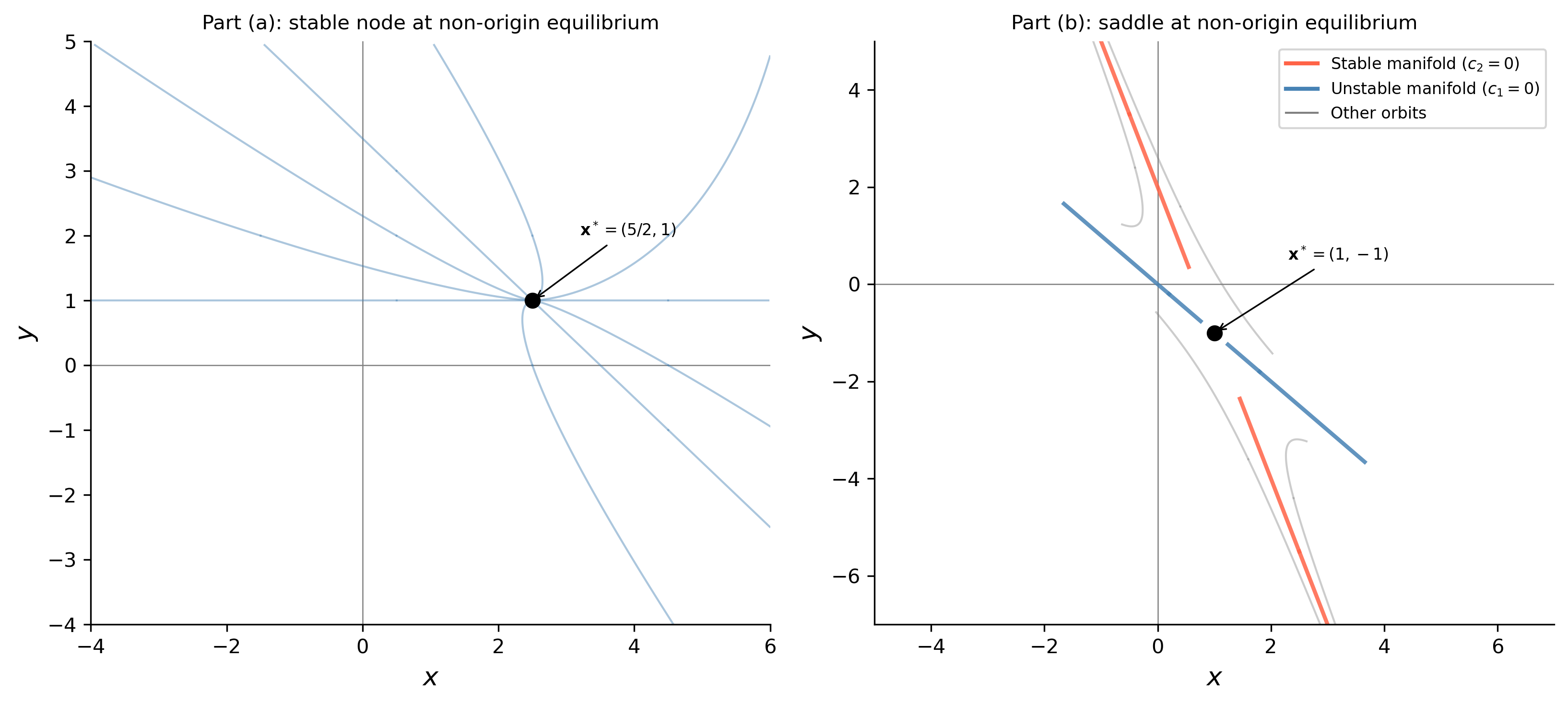
\[ \mathbf{x}^* = \begin{pmatrix}\tfrac{5}{2}\\1\end{pmatrix}. \]

Step 2 — Homogeneous solution of \(\mathbf{u}' = A\mathbf{u}\).

The matrix is upper triangular so eigenvalues are the diagonal entries: \(\lambda_1 = -2\), \(\lambda_2 = -3\).

For \(\lambda_1 = -2\): \((A+2I)\mathbf{v}=\mathbf{0}\) gives \(\begin{pmatrix}0&1\\0&-1\end{pmatrix}\mathbf{v}=\mathbf{0}\), so \(v_2=0\) and \(\mathbf{v}_1=(1,0)^T\).

For \(\lambda_2 = -3\): \((A+3I)\mathbf{v}=\mathbf{0}\) gives \(\begin{pmatrix}1&1\\0&0\end{pmatrix}\mathbf{v}=\mathbf{0}\), so \(v_1=-v_2\) and \(\mathbf{v}_2=(-1,1)^T\).

\[ \mathbf{x}_h(t) = c_1\begin{pmatrix}1\\0\end{pmatrix}e^{-2t} + c_2\begin{pmatrix}-1\\1\end{pmatrix}e^{-3t}. \]

Step 3 — General solution.

\[ \boxed{\mathbf{x}(t) = \begin{pmatrix}\tfrac{5}{2}\\1\end{pmatrix} + c_1\begin{pmatrix}1\\0\end{pmatrix}e^{-2t} + c_2\begin{pmatrix}-1\\1\end{pmatrix}e^{-3t}.} \]

Since both eigenvalues are negative, every trajectory converges to \(\mathbf{x}^*=(\tfrac{5}{2},1)^T\) as \(t\to+\infty\). The equilibrium is an asymptotically stable node.

Part (b).

Step 1 — Equilibrium \(\mathbf{x}^*\).

\[ \begin{pmatrix}2 & 1\\ -3 & -2\end{pmatrix}\mathbf{x}^* = \begin{pmatrix}1\\-1\end{pmatrix}. \]

\(\det A = (2)(-2)-(-3)(1) = -4+3 = -1 \neq 0\), so there is a unique equilibrium.

\[ A^{-1} = \frac{1}{-1}\begin{pmatrix}-2 & -1\\ 3 & 2\end{pmatrix} = \begin{pmatrix}2 & 1\\ -3 & -2\end{pmatrix}. \]

(Note: \(A^{-1} = A\) here, a coincidence for this particular matrix.)

\[ \mathbf{x}^* = A^{-1}\mathbf{b} = \begin{pmatrix}2&1\\-3&-2\end{pmatrix}\begin{pmatrix}1\\-1\end{pmatrix} = \begin{pmatrix}2-1\\-3+2\end{pmatrix} = \begin{pmatrix}1\\-1\end{pmatrix}. \]

Step 2 — Eigenvalues of \(A\).

\(\tau = 2 + (-2) = 0\), \(\delta = -1\). So \(\lambda^2 = 1\), giving \(\lambda = \pm 1\).

Since \(\lambda_1 = -1 < 0 < \lambda_2 = 1\), the equilibrium \(\mathbf{x}^* = (1,-1)^T\) is a saddle point (unstable).

Step 3 — Eigenvectors.

For \(\lambda_1 = -1\): \((A+I)\mathbf{v}=\mathbf{0}\) gives \(\begin{pmatrix}3&1\\-3&-1\end{pmatrix}\mathbf{v}=\mathbf{0}\), so \(3v_1+v_2=0\) and \(\mathbf{v}_1=(1,-3)^T\).

For \(\lambda_2 = 1\): \((A-I)\mathbf{v}=\mathbf{0}\) gives \(\begin{pmatrix}1&1\\-3&-3\end{pmatrix}\mathbf{v}=\mathbf{0}\), so \(v_1+v_2=0\) and \(\mathbf{v}_2=(1,-1)^T\).

Step 4 — General solution.

\[ \boxed{\mathbf{x}(t) = \begin{pmatrix}1\\-1\end{pmatrix} + c_1\begin{pmatrix}1\\-3\end{pmatrix}e^{-t} + c_2\begin{pmatrix}1\\-1\end{pmatrix}e^{t}.} \]

Note

Shifted phase portrait. The phase portrait of the nonhomogeneous system is identical in shape to that of the homogeneous system \(\mathbf{u}' = A\mathbf{u}\), but translated so that the equilibrium is at \(\mathbf{x}^*\) rather than the origin. For part (b) this gives a saddle centered at \((1,-1)\).

Using SymPy

# Part (a)
Aa = sym.Matrix([[-2, 1], [0, -3]])
ba = sym.Matrix([4, 3])
xstar_a = Aa.solve(-ba)
display(Math(r'\text{(a) Equilibrium: }\mathbf{x}^* = ' + sym.latex(xstar_a)))
display(Math(r'\text{(a) Eigenvalues: }' + sym.latex(list(Aa.eigenvals().keys()))))

# Part (b)
Ab = sym.Matrix([[2, 1], [-3, -2]])
bb = sym.Matrix([-1, 1])
xstar_b = Ab.solve(-bb)
display(Math(r'\text{(b) Equilibrium: }\mathbf{x}^* = ' + sym.latex(xstar_b)))
display(Math(r'\text{(b) Eigenvalues: }' + sym.latex(list(Ab.eigenvals().keys()))))

\(\displaystyle \text{(a) Equilibrium: }\mathbf{x}^* = \left[\begin{matrix}\frac{5}{2}\\1\end{matrix}\right]\)

\(\displaystyle \text{(a) Eigenvalues: }\left[ -3, \ -2\right]\)

\(\displaystyle \text{(b) Equilibrium: }\mathbf{x}^* = \left[\begin{matrix}1\\-1\end{matrix}\right]\)

\(\displaystyle \text{(b) Eigenvalues: }\left[ -1, \ 1\right]\)

Show the code

fig, axes = plt.subplots(1, 2, figsize=(11, 5))

# ---- Part (a) ----
ax = axes[0]
xs_a = np.array([5/2, 1])
v1a = np.array([1, 0]); v2a = np.array([-1, 1])
t_f = np.linspace(0, 3, 500); t_b = np.linspace(0, -1, 200)

ax.axhline(0, color='gray', lw=0.6); ax.axvline(0, color='gray', lw=0.6)
for c1v, c2v in [(2,0),(-2,0),(0,2),(0,-2),(1,1),(1,-1),(-1,1),(-1,-1),(3,1),(-3,1)]:
    for tr in [t_f, t_b]:
        xc = xs_a[0] + c1v*v1a[0]*np.exp(-2*tr) + c2v*v2a[0]*np.exp(-3*tr)
        yc = xs_a[1] + c1v*v1a[1]*np.exp(-2*tr) + c2v*v2a[1]*np.exp(-3*tr)
        mask = (np.abs(xc) < 6) & (np.abs(yc) < 5)
        ax.plot(xc[mask], yc[mask], color='steelblue', lw=1.0, alpha=0.45)
ax.plot(*xs_a, 'ko', ms=7, zorder=5)
ax.annotate(r'$\mathbf{x}^*=(5/2,1)$', xy=xs_a, xytext=(3.2, 2.0), fontsize=8,
            arrowprops=dict(arrowstyle='->', color='black', lw=0.8))
ax.set_xlim(-4, 6); ax.set_ylim(-4, 5)
ax.set_xlabel(r'$x$', fontsize=13); ax.set_ylabel(r'$y$', fontsize=13)
ax.set_title('Part (a): stable node at non-origin equilibrium', fontsize=10)

# ---- Part (b) ----
ax = axes[1]
xs_b = np.array([1, -1])
v1b = np.array([1, -3]); v2b = np.array([1, -1])
t_f2 = np.linspace(0,  1.2, 500)
t_b2 = np.linspace(0, -1.2, 500)

ax.axhline(0, color='gray', lw=0.6); ax.axvline(0, color='gray', lw=0.6)
# Stable manifold (c2=0)
for c1v in [1.5, -1.5]:
    for tr in [t_f2, t_b2]:
        xc = xs_b[0] + c1v*v1b[0]*np.exp(-tr)
        yc = xs_b[1] + c1v*v1b[1]*np.exp(-tr)
        mask = (np.abs(xc) < 7) & (np.abs(yc) < 7)
        ax.plot(xc[mask], yc[mask], color='tomato', lw=2.0, alpha=0.85)
# Unstable manifold (c1=0)
for c2v in [0.8, -0.8]:
    for tr in [t_f2, t_b2]:
        xc = xs_b[0] + c2v*v2b[0]*np.exp(tr)
        yc = xs_b[1] + c2v*v2b[1]*np.exp(tr)
        mask = (np.abs(xc) < 7) & (np.abs(yc) < 7)
        ax.plot(xc[mask], yc[mask], color='steelblue', lw=2.0, alpha=0.85)
# Generic orbits
for c1v, c2v in [(1,0.4),(1,-0.4),(-1,0.4),(-1,-0.4)]:
    for tr in [t_f2, t_b2]:
        xc = xs_b[0] + c1v*v1b[0]*np.exp(-tr) + c2v*v2b[0]*np.exp(tr)
        yc = xs_b[1] + c1v*v1b[1]*np.exp(-tr) + c2v*v2b[1]*np.exp(tr)
        mask = (np.abs(xc) < 7) & (np.abs(yc) < 7)
        ax.plot(xc[mask], yc[mask], color='gray', lw=1.0, alpha=0.4)

ax.plot(*xs_b, 'ko', ms=7, zorder=5)
ax.annotate(r'$\mathbf{x}^*=(1,-1)$', xy=xs_b, xytext=(2.3, 0.5), fontsize=8,
            arrowprops=dict(arrowstyle='->', color='black', lw=0.8))
ax.set_xlim(-5, 7); ax.set_ylim(-7, 5)
ax.set_xlabel(r'$x$', fontsize=13); ax.set_ylabel(r'$y$', fontsize=13)
ax.set_title('Part (b): saddle at non-origin equilibrium', fontsize=10)
from matplotlib.lines import Line2D
handles = [Line2D([0],[0], color='tomato',    lw=2, label='Stable manifold ($c_2=0$)'),
           Line2D([0],[0], color='steelblue', lw=2, label='Unstable manifold ($c_1=0$)'),
           Line2D([0],[0], color='gray',      lw=1, label='Other orbits')]
ax.legend(handles=handles, fontsize=8)
plt.tight_layout()
plt.show()

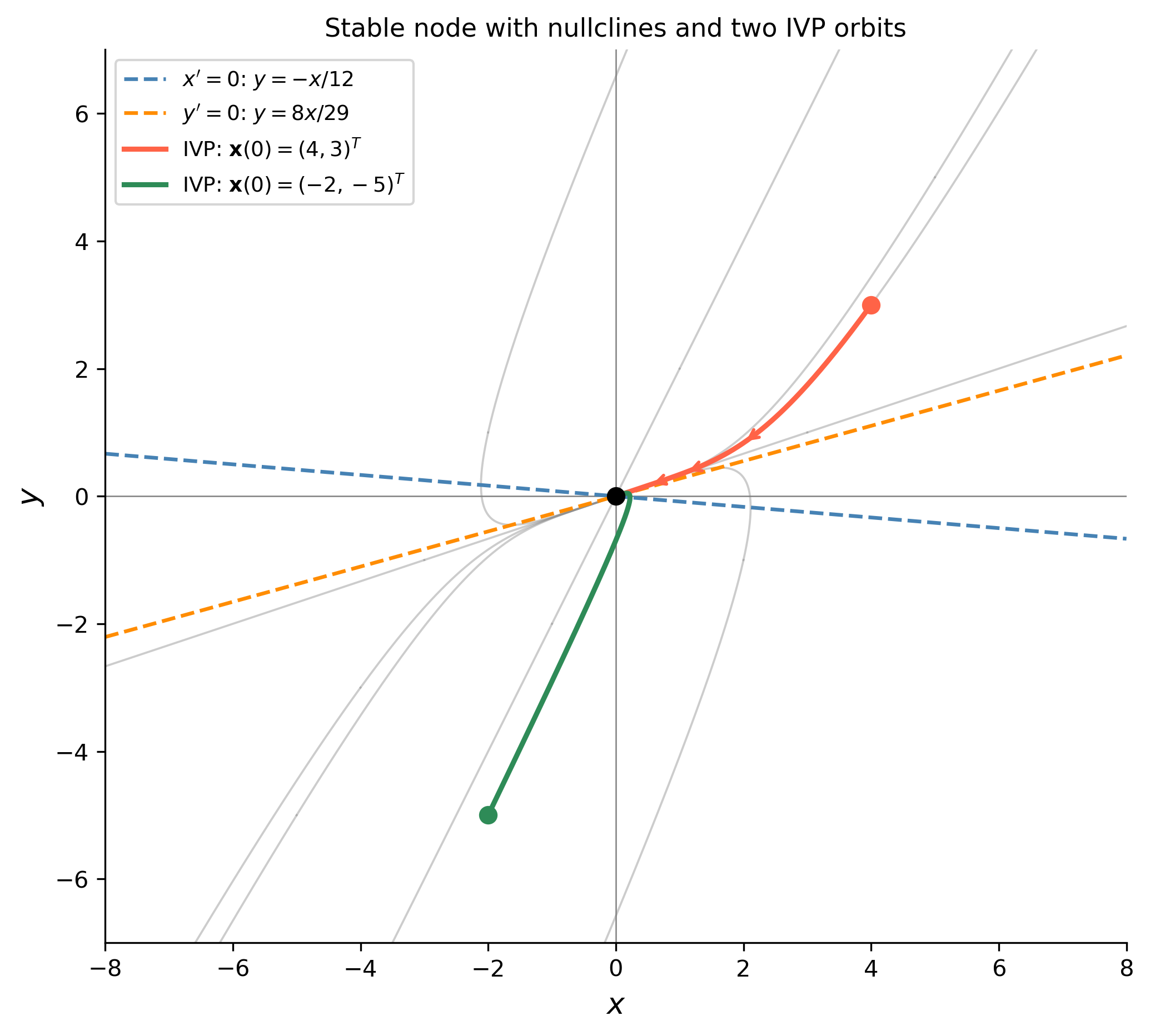
Figure 4: Phase portraits for Example 4. Left (part a): stable node at \(\mathbf{x}^*=(5/2,1)^T\); all orbits converge to the equilibrium. Right (part b): saddle at \(\mathbf{x}^*=(1,-1)^T\); the stable manifold (tomato) and unstable manifold (steelblue) intersect at the equilibrium.

Example 5 — Variation of Parameters with a Given Fundamental Matrix

Consider the nonhomogeneous system \[ \mathbf{x}' = \begin{pmatrix}2 & -1\\ 1 & 0\end{pmatrix}\mathbf{x} + \begin{pmatrix}e^{t}\\ 0\end{pmatrix}. \] It can be verified that a fundamental matrix for the associated homogeneous system is \[ \Phi(t) = \begin{pmatrix}1+t & -t\\ t & 1-t\end{pmatrix}e^{t}. \] Use variation of parameters to find the general solution.

By Hand

Step 1 — Confirm \(\Phi\) is a fundamental matrix.

The two columns of \(\Phi(t)\) should be solutions of \(\mathbf{x}' = A\mathbf{x}\). We check the Wronskian (determinant) to confirm independence:

\[ \det\Phi(t) = e^{2t}\bigl[(1+t)(1-t) - (-t)(t)\bigr] = e^{2t}\bigl[1 - t^2 + t^2\bigr] = e^{2t} \neq 0. \checkmark \]

Step 2 — Compute \(\Phi^{-1}(t)\).

For a \(2\times 2\) matrix \(\Phi = e^{t}\begin{pmatrix}1+t&-t\\t&1-t\end{pmatrix}\):

\[ \Phi^{-1}(t) = \frac{1}{\det\Phi}\begin{pmatrix}1-t & t\\ -t & 1+t\end{pmatrix} = \frac{1}{e^{2t}}\begin{pmatrix}1-t & t\\ -t & 1+t\end{pmatrix} = e^{-2t}\begin{pmatrix}1-t & t\\ -t & 1+t\end{pmatrix}. \]

Step 3 — Compute \(\Phi^{-1}(t)\mathbf{f}(t)\).

\[ \Phi^{-1}(t)\mathbf{f}(t) = e^{-2t}\begin{pmatrix}1-t & t\\ -t & 1+t\end{pmatrix}\begin{pmatrix}e^{t}\\0\end{pmatrix} = e^{-2t}\begin{pmatrix}(1-t)e^{t}\\ -te^{t}\end{pmatrix} = \begin{pmatrix}(1-t)e^{-t}\\ -te^{-t}\end{pmatrix}. \]

Step 4 — Integrate.

\[ \int\Phi^{-1}(t)\mathbf{f}(t)\,dt = \begin{pmatrix}\displaystyle\int(1-t)e^{-t}\,dt\\[6pt] \displaystyle\int -te^{-t}\,dt\end{pmatrix}. \]

Using integration by parts:

\[ \int(1-t)e^{-t}\,dt = -(1-t)e^{-t} - \int e^{-t}\,dt = -(1-t)e^{-t} - e^{-t} = -(2-t)e^{-t}, \]

\[ \int -te^{-t}\,dt = te^{-t} - \int e^{-t}\,dt = te^{-t} + e^{-t} = (t+1)e^{-t}. \]

Omitting the constants of integration (absorbed into \(\mathbf{x}_h\)):

\[ \int\Phi^{-1}(t)\mathbf{f}(t)\,dt = \begin{pmatrix}-(2-t)e^{-t}\\ (t+1)e^{-t}\end{pmatrix}. \]

Step 5 — Particular solution \(\mathbf{x}_p = \Phi(t)\displaystyle\int\Phi^{-1}\mathbf{f}\,dt\).

\[ \mathbf{x}_p = e^{t}\begin{pmatrix}1+t & -t\\ t & 1-t\end{pmatrix} \begin{pmatrix}-(2-t)e^{-t}\\ (t+1)e^{-t}\end{pmatrix} = \begin{pmatrix}(1+t)(-(2-t)) + (-t)(t+1)\\ t(-(2-t)) + (1-t)(t+1)\end{pmatrix}. \]

Compute the first component:

\[ (1+t)(-(2-t)) - t(t+1) = (1+t)\bigl[-(2-t) - t\bigr] = (1+t)(-2) = -2(1+t) = -2 - 2t. \]

Compute the second component:

\[ -t(2-t) + (1-t)(1+t) = -2t + t^2 + 1 - t^2 = 1 - 2t. \]

\[ \mathbf{x}_p = \begin{pmatrix}-2-2t\\ 1-2t\end{pmatrix}. \]

Step 6 — General solution.

\[ \boxed{\mathbf{x}(t) = c_1\begin{pmatrix}1+t\\t\end{pmatrix}e^{t} + c_2\begin{pmatrix}-t\\1-t\end{pmatrix}e^{t} + \begin{pmatrix}-2-2t\\ 1-2t\end{pmatrix}.} \]

Note

Structure of the particular solution. Note that \(\mathbf{x}_p\) is a linear polynomial in \(t\) (no \(e^t\) factor), even though the forcing \(\mathbf{f}(t)=e^t(1,0)^T\) contains \(e^t\). This is because \(e^t\) is already a growth rate built into the homogeneous solutions; the variation of parameters formula accounts for this automatically — unlike undetermined coefficients, it requires no modification rule.

Using SymPy

t = sym.Symbol('t')

A5 = sym.Matrix([[2, -1], [1, 0]])
f5 = sym.Matrix([sym.exp(t), 0])

Phi5 = sym.Matrix([[(1+t)*sym.exp(t), -t*sym.exp(t)],
                   [t*sym.exp(t),      (1-t)*sym.exp(t)]])

display(Math(r'\det\Phi = ' + sym.latex(sym.simplify(Phi5.det()))))

Phi5_inv = sym.simplify(Phi5.inv())
display(Math(r'\Phi^{-1}(t) = ' + sym.latex(Phi5_inv)))

integrand = sym.simplify(Phi5_inv * f5)
display(Math(r'\Phi^{-1}\mathbf{f} = ' + sym.latex(integrand)))

integral = sym.integrate(integrand, t)
display(Math(r'\int\Phi^{-1}\mathbf{f}\,dt = ' + sym.latex(sym.simplify(integral))))

xp = sym.simplify(Phi5 * integral)
display(Math(r'\mathbf{x}_p = ' + sym.latex(xp)))

\(\displaystyle \det\Phi = e^{2 t}\)

\(\displaystyle \Phi^{-1}(t) = \left[\begin{matrix}\left(1 - t\right) e^{- t} & t e^{- t}\\- t e^{- t} & \left(t + 1\right) e^{- t}\end{matrix}\right]\)

\(\displaystyle \Phi^{-1}\mathbf{f} = \left[\begin{matrix}1 - t\\- t\end{matrix}\right]\)

\(\displaystyle \int\Phi^{-1}\mathbf{f}\,dt = \left[\begin{matrix}\frac{t \left(2 - t\right)}{2}\\- \frac{t^{2}}{2}\end{matrix}\right]\)

\(\displaystyle \mathbf{x}_p = \left[\begin{matrix}\frac{t \left(t + 2\right) e^{t}}{2}\\\frac{t^{2} e^{t}}{2}\end{matrix}\right]\)

Example 6 — Undetermined Coefficients for a System

Find a particular solution of \[ \mathbf{x}' = \begin{pmatrix}-5 & 3\\ 2 & -10\end{pmatrix}\mathbf{x} + \begin{pmatrix}e^{-t}\\ 2e^{-t}\end{pmatrix}. \]

By Hand

Step 1 — Check that \(e^{-t}\) is not a homogeneous solution.

The eigenvalues of \(A = \begin{pmatrix}-5&3\\2&-10\end{pmatrix}\) satisfy

\[ \lambda^2 + 15\lambda + 44 = (\lambda+4)(\lambda+11) = 0, \quad\Longrightarrow\quad \lambda_1 = -4,\;\lambda_2 = -11. \]

Since \(-1\) is not an eigenvalue, the forcing rate \(e^{-t}\) does not duplicate any homogeneous solution. We may use the standard (unmodified) trial form.

Step 2 — Trial particular solution.

Since both forcing components are proportional to \(e^{-t}\), try

\[ \mathbf{x}_p = \mathbf{a}\,e^{-t} = \begin{pmatrix}a_1\\a_2\end{pmatrix}e^{-t}. \]

Step 3 — Substitute into \(\mathbf{x}' = A\mathbf{x} + \mathbf{f}\).

\[ \mathbf{x}_p' = -\mathbf{a}\,e^{-t}. \]

Substituting:

\[ -\mathbf{a}\,e^{-t} = A\mathbf{a}\,e^{-t} + \begin{pmatrix}1\\2\end{pmatrix}e^{-t}. \]

Divide through by \(e^{-t}\):

\[ -\mathbf{a} = A\mathbf{a} + \begin{pmatrix}1\\2\end{pmatrix} \quad\Longrightarrow\quad (A + I)\mathbf{a} = -\begin{pmatrix}1\\2\end{pmatrix}. \]

Step 4 — Solve \((A+I)\mathbf{a} = -(1,2)^T\).

\[ A + I = \begin{pmatrix}-4 & 3\\ 2 & -9\end{pmatrix}. \]

\(\det(A+I) = (-4)(-9) - (3)(2) = 36 - 6 = 30.\)

By Cramer’s rule:

\[ a_1 = \frac{\det\begin{pmatrix}-1&3\\-2&-9\end{pmatrix}}{30} = \frac{9+6}{30} = \frac{15}{30} = \frac{1}{2}, \]

\[ a_2 = \frac{\det\begin{pmatrix}-4&-1\\2&-2\end{pmatrix}}{30} = \frac{8+2}{30} = \frac{10}{30} = \frac{1}{3}. \]

Step 5 — Particular solution.

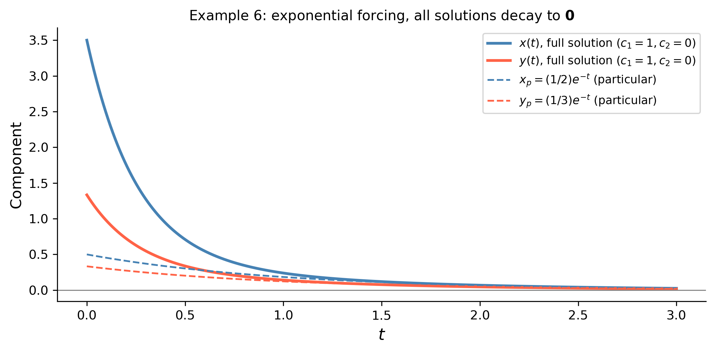
\[ \boxed{\mathbf{x}_p = \begin{pmatrix}\tfrac{1}{2}\\[4pt]\tfrac{1}{3}\end{pmatrix}e^{-t}.} \]

Step 6 — Eigenvectors for the general solution.

For \(\lambda_1 = -4\): \((A+4I)\mathbf{v}=\mathbf{0}\) gives \(\begin{pmatrix}-1&3\\2&-6\end{pmatrix}\mathbf{v}=\mathbf{0}\), so \(v_1=3v_2\) and \(\mathbf{v}_1=(3,1)^T\).

For \(\lambda_2 = -11\): \((A+11I)\mathbf{v}=\mathbf{0}\) gives \(\begin{pmatrix}6&3\\2&1\end{pmatrix}\mathbf{v}=\mathbf{0}\), so \(v_1=-\tfrac{1}{2}v_2\) and \(\mathbf{v}_2=(1,-2)^T\).

The complete general solution is

\[ \boxed{\mathbf{x}(t) = c_1\begin{pmatrix}3\\1\end{pmatrix}e^{-4t} + c_2\begin{pmatrix}1\\-2\end{pmatrix}e^{-11t} + \begin{pmatrix}\tfrac{1}{2}\\ \tfrac{1}{3}\end{pmatrix}e^{-t}.} \]

Tip

Long-run behavior. As \(t \to +\infty\), both homogeneous terms decay (\(e^{-4t}\) and \(e^{-11t}\) both \(\to 0\)), but the particular solution \((\tfrac{1}{2},\tfrac{1}{3})^T e^{-t}\) also decays to zero. So all solutions approach \(\mathbf{0}\), reflecting the fact that the origin is the only equilibrium of the unforced system and the forcing itself decays. If the forcing were a nonzero constant \(\mathbf{b}\) instead, solutions would converge to a nonzero equilibrium \(-A^{-1}\mathbf{b}\).

Using SymPy

A6 = sym.Matrix([[-5, 3], [2, -10]])
f6 = sym.Matrix([sym.exp(-t), 2*sym.exp(-t)])

display(Math(r'\text{Eigenvalues of }A: '
            + sym.latex(list(A6.eigenvals().keys()))))

# Trial: x_p = a*e^{-t}; solve (A+I)a = -(1,2)^T
rhs6 = sym.Matrix([-1, -2])
a_vec = (A6 + sym.eye(2)).solve(rhs6)
display(Math(r'\mathbf{a} = ' + sym.latex(a_vec)))

xp6 = a_vec * sym.exp(-t)
display(Math(r'\mathbf{x}_p = ' + sym.latex(xp6)))

# Verify
lhs_check = sym.diff(xp6, t) - A6*xp6 - f6
display(Math(r'\mathbf{x}_p\prime - A\mathbf{x}_p - \mathbf{f} = '
            + sym.latex(sym.simplify(lhs_check))
            + r'\quad\checkmark'))

\(\displaystyle \text{Eigenvalues of }A: \left[ -4, \ -11\right]\)

\(\displaystyle \mathbf{a} = \left[\begin{matrix}\frac{1}{2}\\\frac{1}{3}\end{matrix}\right]\)

\(\displaystyle \mathbf{x}_p = \left[\begin{matrix}\frac{e^{- t}}{2}\\\frac{e^{- t}}{3}\end{matrix}\right]\)

\(\displaystyle \mathbf{x}_p\prime - A\mathbf{x}_p - \mathbf{f} = \left[\begin{matrix}0\\0\end{matrix}\right]\quad\checkmark\)

Show the code

t_vals = np.linspace(0, 3, 500)

# Particular solution
xp_x = 0.5 * np.exp(-t_vals)
xp_y = (1/3) * np.exp(-t_vals)

# Complete solution: c1=1, c2=0
x_full = 3*np.exp(-4*t_vals) + 0.5*np.exp(-t_vals)
y_full = 1*np.exp(-4*t_vals) + (1/3)*np.exp(-t_vals)

fig, ax = plt.subplots(figsize=(8, 4))
ax.plot(t_vals, x_full, color='steelblue', lw=2.2,
        label=r'$x(t)$, full solution ($c_1=1,c_2=0$)')
ax.plot(t_vals, y_full, color='tomato', lw=2.2,
        label=r'$y(t)$, full solution ($c_1=1,c_2=0$)')
ax.plot(t_vals, xp_x, color='steelblue', lw=1.4, ls='--',
        label=r'$x_p = (1/2)e^{-t}$ (particular)')
ax.plot(t_vals, xp_y, color='tomato', lw=1.4, ls='--',
        label=r'$y_p = (1/3)e^{-t}$ (particular)')
ax.axhline(0, color='gray', lw=0.8)
ax.set_xlabel(r'$t$', fontsize=13)
ax.set_ylabel('Component', fontsize=12)
ax.set_title(r'Example 6: exponential forcing, all solutions decay to $\mathbf{0}$',
             fontsize=11)
ax.legend(fontsize=9)
plt.tight_layout()
plt.show()

Figure 5: Time-series plot for Example 6 showing \(x(t)\) (steelblue) and \(y(t)\) (tomato) for the particular solution \(\mathbf{x}_p = (\tfrac{1}{2}, \tfrac{1}{3})^T e^{-t}\) (dashed) and the complete solution with \(c_1=1\), \(c_2=0\) (solid). Both decay to zero as \(t\to+\infty\).

References

Logan, J David. 2015. A First Course in Differential Equations, Third Edition.

Expand for Session Info

import sys
print("Python version:", sys.version)
print('\n'.join(f'{m.__name__}=={m.__version__}'
                for m in globals().values()
                if getattr(m, '__version__', None)))

Python version: 3.14.4 | packaged by conda-forge | (main, Apr  8 2026, 02:33:53) [Clang 20.1.8 ]
numpy==2.4.3
sympy==1.14.0
matplotlib==3.10.8

Reuse

CC BY-NC-SA 4.0