Numerical Methods for ODEs — Worked Examples

Show the code
# This is a code cell that imports the necessary libraries for our session.
import numpy as np                        # NumPy for numerical computations
import sympy as sym                       # SymPy for symbolic mathematics
import matplotlib as mpl                  # Matplotlib for plotting
import matplotlib.pyplot as plt           # Matplotlib pyplot interface
from scipy.integrate import solve_ivp     # SciPy ODE solver (for verification)
from IPython.display import Math, display
mpl.rcParams['figure.dpi'] = 150
mpl.rcParams['axes.spines.top'] = False
mpl.rcParams['axes.spines.right'] = False

In this document we work through fully solved examples for the topics covered in Sections 6.2 and 6.3 of the text (Logan 2015):

Each example is worked step-by-step by hand (showing one or two explicit steps of the algorithm) and then carried to completion with Python. Every numerical solution is compared with either the exact solution or a high-accuracy reference computed by SciPy’s solve_ivp.


§6.2 Numerical Methods for a Single ODE

Given a first-order IVP \(x' = f(t, x)\), \(x(t_0) = x_0\), on \([t_0, T]\) with step size \(h\) and \(N = (T - t_0)/h\) steps, the three methods produce a sequence of approximations \(X_0, X_1, \ldots, X_N \approx x(t_0), x(t_1), \ldots, x(t_N)\).

Euler method (order \(h\)):

\[X_{n+1} = X_n + h\,f(t_n, X_n).\]

Modified Euler (Heun) method (order \(h^2\)):

\[ k_1 = f(t_n, X_n), \qquad k_2 = f(t_n + h,\; X_n + h k_1), \qquad X_{n+1} = X_n + \frac{h}{2}(k_1 + k_2). \]

Runge–Kutta method (order \(h^4\)):

\[ k_1 = f(t_n, X_n), \quad k_2 = f\!\left(t_n+\tfrac{h}{2}, X_n+\tfrac{h}{2}k_1\right), \quad k_3 = f\!\left(t_n+\tfrac{h}{2}, X_n+\tfrac{h}{2}k_2\right), \quad k_4 = f(t_n+h, X_n+hk_3), \] \[ X_{n+1} = X_n + \frac{h}{6}(k_1 + 2k_2 + 2k_3 + k_4). \]


Example 1 — Comparing All Three Methods on a Linear IVP

Consider the initial value problem \[ x' = x - 2t, \qquad x(0) = 1, \] on the interval \(0 \le t \le 2\).

(a) Use the Euler method and the modified Euler method with step size \(h = 0.5\) to approximate the solution, and compare both with the exact answer at \(t = 2\). (b) Apply the Runge–Kutta method with \(h = 0.5\) and confirm its superior accuracy. (c) Using step sizes \(h = 0.1\), \(h = 0.01\), and \(h = 0.001\), verify numerically that the cumulative error at \(t = 2\) is \(O(h)\) for Euler, \(O(h^2)\) for modified Euler, and \(O(h^4)\) for RK4.

Exact Solution

The ODE \(x' - x = -2t\) is linear with integrating factor \(e^{-t}\).

\[ \frac{d}{dt}\!\left(e^{-t}x\right) = -2te^{-t} \implies e^{-t}x = -2\int te^{-t}\,dt = 2e^{-t}(t+1) + C. \]

Applying \(x(0)=1\): \(1 = 2 + C\), so \(C = -1\).

\[ \boxed{x(t) = 2t + 2 - e^t.} \]

At \(t = 2\): \(x(2) = 4 + 2 - e^2 = 6 - e^2 \approx -1.3891\).

By Hand — Two Euler Steps

Here \(f(t,x) = x - 2t\), \(h = 0.5\), \(X_0 = 1\).

Step 0 → 1 (\(t_0 = 0\), \(X_0 = 1\)): \[ X_1 = X_0 + h f(0, 1) = 1 + 0.5(1 - 0) = 1.5. \] Exact: \(x(0.5) = 1 + 2 - e^{0.5} \approx 1.3513\). Error \(\approx 0.1487\).

Step 1 → 2 (\(t_1 = 0.5\), \(X_1 = 1.5\)): \[ X_2 = 1.5 + 0.5(1.5 - 1.0) = 1.5 + 0.25 = 1.75. \] Exact: \(x(1) = 2 + 2 - e^1 \approx 1.2817\). Error \(\approx 0.4683\).

By Hand — Two Modified Euler Steps

Step 0 → 1:

\[ k_1 = f(0, 1) = 1,\qquad k_2 = f(0.5,\; 1 + 0.5\cdot1) = f(0.5, 1.5) = 1.5 - 1 = 0.5. \] \[ X_1 = 1 + \frac{0.5}{2}(1 + 0.5) = 1 + 0.375 = 1.375. \] Exact: \(1.3513\). Error \(\approx 0.0237\) — already much smaller than Euler.

By Hand — One RK4 Step

Step 0 → 1 (\(h = 0.5\), \((t_0, X_0) = (0, 1)\)):

\[ k_1 = f(0,\,1) = 1, \] \[ k_2 = f(0.25,\,1.25) = 1.25 - 0.5 = 0.75, \] \[ k_3 = f(0.25,\,1 + 0.25\cdot0.75) = f(0.25,\,1.1875) = 1.1875 - 0.5 = 0.6875, \] \[ k_4 = f(0.5,\,1 + 0.5\cdot0.6875) = f(0.5,\,1.34375) = 1.34375 - 1 = 0.34375. \] \[ X_1 = 1 + \frac{0.5}{6}(1 + 2(0.75) + 2(0.6875) + 0.34375) = 1 + \frac{0.5}{6}(4.21875) \approx 1.3516. \] Exact: \(1.3513\). Error \(\approx 0.0003\) — already nearly exact with a single step!

Tip

Reading accuracy from the by-hand steps. With \(h = 0.5\), the Euler error is \(\sim 0.15\), the modified Euler error is \(\sim 0.02\) (about \(8\times\) smaller), and the RK4 error is \(\sim 0.0003\) (about \(500\times\) smaller). This illustrates the dramatic improvement from first-order to second-order to fourth-order methods even at a coarse step size.

Python Implementation and Error Study

def euler(f, t0, x0, T, h):
    """Euler method for x' = f(t,x), returns (t_arr, X_arr)."""
    ts = [t0]; xs = [x0]
    t, x = t0, x0
    while t < T - 1e-12:
        x = x + h * f(t, x)
        t = t + h
        ts.append(t); xs.append(x)
    return np.array(ts), np.array(xs)

def modified_euler(f, t0, x0, T, h):
    """Modified Euler (Heun) method."""
    ts = [t0]; xs = [x0]
    t, x = t0, x0
    while t < T - 1e-12:
        k1 = f(t, x)
        k2 = f(t + h, x + h * k1)
        x  = x + (h / 2) * (k1 + k2)
        t  = t + h
        ts.append(t); xs.append(x)
    return np.array(ts), np.array(xs)

def rk4(f, t0, x0, T, h):
    """Classical Runge–Kutta (RK4) method."""
    ts = [t0]; xs = [x0]
    t, x = t0, x0
    while t < T - 1e-12:
        k1 = f(t,           x)
        k2 = f(t + h/2,     x + (h/2)*k1)
        k3 = f(t + h/2,     x + (h/2)*k2)
        k4 = f(t + h,       x + h*k3)
        x  = x + (h/6)*(k1 + 2*k2 + 2*k3 + k4)
        t  = t + h
        ts.append(t); xs.append(x)
    return np.array(ts), np.array(xs)

# IVP definition
f1   = lambda t, x: x - 2*t
x_exact1 = lambda t: 2*t + 2 - np.exp(t)
t0, x0, T = 0.0, 1.0, 2.0

# Solve with h = 0.5 for comparison
h = 0.5
t_e,  X_e  = euler(f1, t0, x0, T, h)
t_me, X_me = modified_euler(f1, t0, x0, T, h)
t_rk, X_rk = rk4(f1, t0, x0, T, h)

print(f"Exact x(2)           = {x_exact1(2):.6f}")
print(f"Euler x(2)           = {X_e[-1]:.6f}  (error {abs(X_e[-1]-x_exact1(2)):.6f})")
print(f"Modified Euler x(2)  = {X_me[-1]:.6f}  (error {abs(X_me[-1]-x_exact1(2)):.6f})")
print(f"RK4 x(2)             = {X_rk[-1]:.6f}  (error {abs(X_rk[-1]-x_exact1(2)):.2e})")
Exact x(2)           = -1.389056
Euler x(2)           = 0.937500  (error 2.326556)
Modified Euler x(2)  = -0.972900  (error 0.416156)
RK4 x(2)             = -1.383970  (error 5.09e-03)
# Error at t=2 for several step sizes
step_sizes = [0.1, 0.01, 0.001, 0.0001]
exact_T = x_exact1(T)

print(f"{'h':>8}  {'Euler err':>12}  {'Mod.Euler err':>14}  {'RK4 err':>12}")
print("-" * 54)
for h in step_sizes:
    _, Xe  = euler(f1, t0, x0, T, h)
    _, Xme = modified_euler(f1, t0, x0, T, h)
    _, Xrk = rk4(f1, t0, x0, T, h)
    print(f"{h:>8.4f}  {abs(Xe[-1]-exact_T):>12.2e}  "
          f"{abs(Xme[-1]-exact_T):>14.2e}  {abs(Xrk[-1]-exact_T):>12.2e}")
       h     Euler err   Mod.Euler err       RK4 err
------------------------------------------------------
  0.1000      6.62e-01        2.28e-02      1.13e-05
  0.0100      7.30e-02        2.44e-04      1.22e-09
  0.0010      7.38e-03        2.46e-06      2.82e-13
  0.0001      7.39e-04        2.46e-08      7.73e-13
Show the code
fig, axes = plt.subplots(1, 2, figsize=(11, 5))

# Left: solution comparison
ax = axes[0]
t_fine = np.linspace(0, 2, 400)
ax.plot(t_fine, x_exact1(t_fine), 'k-',  lw=2.2, label='Exact', zorder=5)
ax.plot(t_e,  X_e,  'o--', color='tomato',    lw=1.5, ms=6, label='Euler ($h=0.5$)')
ax.plot(t_me, X_me, 's--', color='darkorange', lw=1.5, ms=6, label='Mod. Euler ($h=0.5$)')
ax.plot(t_rk, X_rk, '^--', color='steelblue',  lw=1.5, ms=6, label='RK4 ($h=0.5$)')
ax.set_xlabel(r'$t$', fontsize=13)
ax.set_ylabel(r'$x$', fontsize=13)
ax.set_title(r"$x' = x - 2t$, $x(0) = 1$", fontsize=11)
ax.legend(fontsize=9)

# Right: error convergence
ax = axes[1]
hs  = np.array([0.2, 0.1, 0.05, 0.025, 0.01])
err_e = []; err_me = []; err_rk = []
for h in hs:
    _, Xe  = euler(f1, t0, x0, T, h)
    _, Xme = modified_euler(f1, t0, x0, T, h)
    _, Xrk = rk4(f1, t0, x0, T, h)
    err_e.append(abs(Xe[-1]  - exact_T))
    err_me.append(abs(Xme[-1] - exact_T))
    err_rk.append(abs(Xrk[-1] - exact_T))

ax.loglog(hs, err_e,  'o-', color='tomato',    lw=1.8, ms=7, label='Euler')
ax.loglog(hs, err_me, 's-', color='darkorange', lw=1.8, ms=7, label='Mod. Euler')
ax.loglog(hs, err_rk, '^-', color='steelblue',  lw=1.8, ms=7, label='RK4')

# Reference slopes
ax.loglog(hs, 3*hs,       'k:',  lw=1.2, label=r'$O(h)$')
ax.loglog(hs, 4*hs**2,    'k--', lw=1.2, label=r'$O(h^2)$')
ax.loglog(hs, 0.1*hs**4,  'k-.',  lw=1.2, label=r'$O(h^4)$')
ax.set_xlabel(r'Step size $h$', fontsize=13)
ax.set_ylabel(r'$|X_N - x(2)|$', fontsize=13)
ax.set_title('Error convergence at $t=2$', fontsize=11)
ax.legend(fontsize=8)

plt.suptitle(r"Example 1: $x'=x-2t$, $x(0)=1$", fontsize=11)
plt.tight_layout()
plt.show()
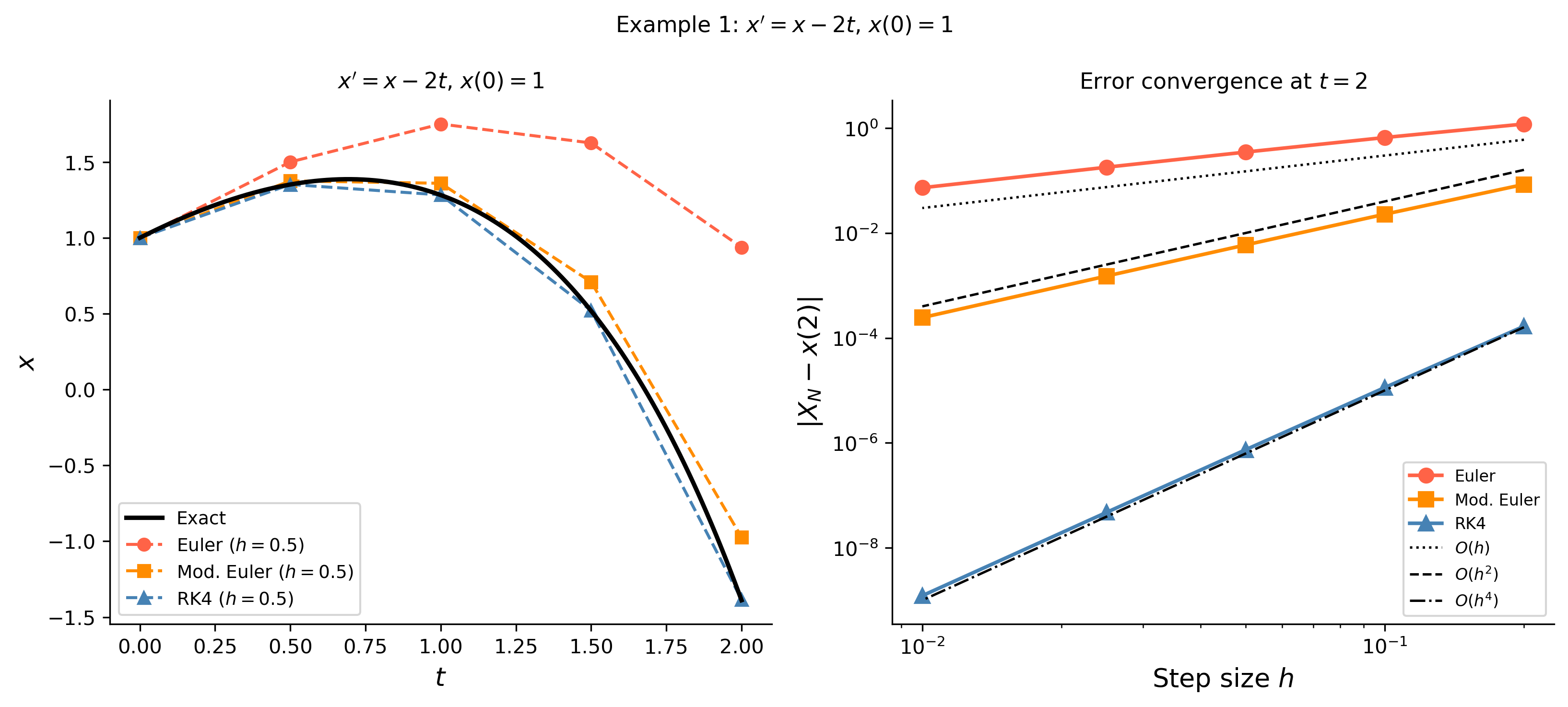
Figure 1: Example 1. Left: solutions for \(h=0.5\) compared to the exact curve; the Euler method drifts visibly while modified Euler and RK4 track closely. Right: log–log error plot at \(t=2\) confirming \(O(h)\), \(O(h^2)\), and \(O(h^4)\) convergence rates.

Example 2 — Stiff-Like Behaviour: When Step Size Matters

Consider the IVP \[ x' = -5x + 5\cos t + \sin t, \qquad x(0) = 0, \] on \(0 \le t \le 10\).

(a) Find the exact solution. (b) Use the Euler method with \(N = 30\), \(100\), \(300\), and \(1000\) steps. Comment on the accuracy and on what happens for small \(N\).

Exact Solution

The ODE is linear: \(x' + 5x = 5\cos t + \sin t\). Integrating factor \(e^{5t}\):

\[ \frac{d}{dt}(e^{5t}x) = e^{5t}(5\cos t + \sin t). \]

Using \(\int e^{5t}\cos t\,dt = \frac{e^{5t}(5\cos t + \sin t)}{26}\) and \(\int e^{5t}\sin t\,dt = \frac{e^{5t}(5\sin t - \cos t)}{26}\):

\[ e^{5t}x = \frac{e^{5t}}{26}(25\cos t + 5\sin t + 5\sin t - \cos t) + C = \frac{e^{5t}}{26}(24\cos t + 10\sin t) + C. \]

Applying \(x(0) = 0\): \(0 = \tfrac{24}{26} + C\), so \(C = -\tfrac{12}{13}\).

\[ \boxed{x(t) = \cos t + \frac{2}{5}\sin t - \frac{12}{13}e^{-5t}.} \]

For large \(t\) the transient term \(e^{-5t}\) vanishes and the solution approaches the steady state \(x_{\rm ss}(t) = \cos t + \tfrac{2}{5}\sin t\).

Note

Why step size matters here. The homogeneous solution decays like \(e^{-5t}\), which has a “time constant” of \(1/5 = 0.2\). The Euler method is stable only when \(|1 + h\lambda| \le 1\) for the dominant eigenvalue \(\lambda = -5\), requiring \(h \le 2/5 = 0.4\). With \(N = 30\) steps over \([0, 10]\) we get \(h = 1/3 \approx 0.33\), which is just inside the stability boundary; smaller step sizes are much safer and more accurate.

Show the code
f2 = lambda t, x: -5*x + 5*np.cos(t) + np.sin(t)
x_exact2 = lambda t: np.cos(t) + 0.4*np.sin(t) - (12/13)*np.exp(-5*t)
t0, x0, T2 = 0.0, 0.0, 10.0

fig, ax = plt.subplots(figsize=(9, 5))
t_fine = np.linspace(0, T2, 1000)
ax.plot(t_fine, x_exact2(t_fine), 'k-', lw=2.5, label='Exact', zorder=10)

for N, col, alpha in [(30, 'tomato', 0.9), (100, 'darkorange', 0.8),
                       (300, 'steelblue', 0.75), (1000, 'seagreen', 0.7)]:
    h = T2 / N
    te, Xe = euler(f2, t0, x0, T2, h)
    ax.plot(te, Xe, lw=1.4, alpha=alpha, color=col,
            label=f'Euler $N={N}$ ($h={h:.3f}$)')

ax.set_xlim(0, T2)
ax.set_ylim(-1.8, 2.0)
ax.set_xlabel(r'$t$', fontsize=13)
ax.set_ylabel(r'$x$', fontsize=13)
ax.set_title(r"$x' = -5x + 5\cos t + \sin t$, $x(0)=0$", fontsize=11)
ax.legend(fontsize=9)
plt.tight_layout()
plt.show()
Figure 2: Example 2. Euler solutions with \(N=30\) (very coarse, unstable-looking), \(N=100\), \(N=300\), and \(N=1000\) steps, compared to the exact solution. The coarse grid fails to capture the rapid transient. Finer grids converge to the exact curve.

Example 3 — Logistic Growth with Periodic Harvesting

A fish population (in thousands) is modelled by \[ x' = 0.4x\!\left(1 - \frac{x}{8}\right) - 0.3\sin^2(\pi t/6), \qquad x(0) = 3, \] where time \(t\) is in months and the harvesting term varies seasonally. Use the Euler method to plot the population over 5 years (60 months).

Note

There is no closed-form exact solution here. Numerical methods are the only practical approach.

Analysis of the Equation

Without harvesting the equation is logistic with intrinsic growth rate \(r = 0.4\) and carrying capacity \(K = 8\) (thousand fish). The harvesting term \(0.3\sin^2(\pi t/6)\) is always non-negative, oscillates between \(0\) and \(0.3\) with period 12 months (simulating summer/winter fishing seasons), and has mean value \(0.15\).

The equilibrium of the unforced logistic equation is \(K = 8\). With average harvesting \(0.15\), we expect the long-term average population to settle below 8 but to oscillate around a new pseudo-equilibrium.

By Hand — First Two Euler Steps

\(f(t, x) = 0.4x(1 - x/8) - 0.3\sin^2(\pi t/6)\), \(h = 1\) month, \(X_0 = 3\).

Step 0 → 1: \[ f(0, 3) = 0.4(3)(1 - 3/8) - 0 = 1.2 \cdot 0.625 = 0.75. \] \[ X_1 = 3 + 1 \cdot 0.75 = 3.75. \]

Step 1 → 2: \[ f(1, 3.75) = 0.4(3.75)(1 - 3.75/8) - 0.3\sin^2(\pi/6) = 1.5(0.53125) - 0.3(0.25) \approx 0.7969 - 0.075 = 0.7219. \] \[ X_2 = 3.75 + 0.7219 = 4.472. \]

Show the code
f3 = lambda t, x: 0.4*x*(1 - x/8) - 0.3*np.sin(np.pi*t/6)**2
t0, x0, T3 = 0.0, 3.0, 60.0

h = 0.5
te3, Xe3 = euler(f3, t0, x0, T3, h)

fig, ax = plt.subplots(figsize=(9, 4))
ax.plot(te3, Xe3, color='steelblue', lw=1.8, label='Euler ($h=0.5$ months)')
ax.axhline(8.0, color='gray', ls='--', lw=1.2, label='Carrying capacity $K=8$')
ax.axhline(np.mean(Xe3[len(Xe3)//2:]), color='tomato', ls=':', lw=1.5,
           label=f'Long-term mean ≈ {np.mean(Xe3[len(Xe3)//2:]):.2f}')
ax.set_xlabel(r'$t$ (months)', fontsize=13)
ax.set_ylabel(r'Population (thousands)', fontsize=13)
ax.set_title(r'Logistic growth with seasonal harvesting: $x(0)=3$', fontsize=11)
ax.legend(fontsize=9)
plt.tight_layout()
plt.show()
Figure 3: Example 3. Euler solution for logistic growth with seasonal harvesting, \(h=0.5\) months over 60 months (5 years). The population rises from 3, oscillates seasonally, and fluctuates around a long-term average well below the unharvested carrying capacity \(K=8\).

§6.3 Systems of Equations

For a \(2\times 2\) system \(x' = f(t, x, y)\), \(y' = g(t, x, y)\) with initial conditions \(x(t_0)=x_0\), \(y(t_0)=y_0\), the Runge–Kutta formulas become those on pp. 329–330 of the text, involving eight slopes \(k_{11}, k_{21}, \ldots, k_{24}\).


Example 4 — Coupled Linear System: Full RK4 by Hand

Solve the initial value problem \[ x' = -x + y, \qquad y' = -y, \qquad x(0) = 2,\; y(0) = 1, \] numerically on \([0, 3]\) using RK4 with \(h = 0.5\). Compare with the exact solution.

Exact Solution

The \(y\)-equation is decoupled: \(y' = -y \implies y(t) = e^{-t}\).

The \(x\)-equation becomes \(x' = -x + e^{-t}\), which is linear: integrating factor \(e^t\) gives

\[ \frac{d}{dt}(e^t x) = e^t(-x + e^{-t}) \cdot e^t / e^t = 1 \;\Longrightarrow\; e^t x = t + C. \]

Applying \(x(0) = 2\): \(C = 2\).

\[ \boxed{x(t) = (t + 2)e^{-t}, \qquad y(t) = e^{-t}.} \]

By Hand — One RK4 Step

With \(f = -x + y\) and \(g = -y\), \(h = 0.5\), \((t_0, X_0, Y_0) = (0, 2, 1)\):

\[ k_{11} = f(0, 2, 1) = -2 + 1 = -1, \qquad k_{21} = g(0, 2, 1) = -1. \] \[ k_{12} = f\!\left(0.25,\; 2 + 0.25(-1),\; 1 + 0.25(-1)\right) = f(0.25, 1.75, 0.75) = -1.75 + 0.75 = -1.00, \] \[ k_{22} = g(0.25, 1.75, 0.75) = -0.75. \] \[ k_{13} = f(0.25,\; 2 + 0.25(-1),\; 1 + 0.25(-0.75)) = f(0.25, 1.75, 0.8125) = -1.75 + 0.8125 = -0.9375, \] \[ k_{23} = g(0.25, 1.75, 0.8125) = -0.8125. \] \[ k_{14} = f(0.5,\; 2 + 0.5(-0.9375),\; 1 + 0.5(-0.8125)) = f(0.5, 1.53125, 0.59375) = -1.53125 + 0.59375 = -0.9375, \] \[ k_{24} = g(0.5, 1.53125, 0.59375) = -0.59375. \]

\[ X_1 = 2 + \frac{0.5}{6}(-1 + 2(-1) + 2(-0.9375) + (-0.9375)) = 2 + \frac{0.5}{6}(-5.8125) \approx 2 - 0.4844 = 1.5156. \]

Exact: \(x(0.5) = (2.5)e^{-0.5} \approx 1.5163\). Error \(\approx 0.0007\).

def rk4_system(f, g, t0, x0, y0, T, h):
    """RK4 for the 2x2 system x'=f(t,x,y), y'=g(t,x,y)."""
    ts = [t0]; xs = [x0]; ys = [y0]
    t, x, y = t0, x0, y0
    while t < T - 1e-12:
        k11 = f(t, x, y);            k21 = g(t, x, y)
        k12 = f(t+h/2, x+h/2*k11, y+h/2*k21)
        k22 = g(t+h/2, x+h/2*k11, y+h/2*k21)
        k13 = f(t+h/2, x+h/2*k12, y+h/2*k22)
        k23 = g(t+h/2, x+h/2*k12, y+h/2*k22)
        k14 = f(t+h,   x+h*k13,   y+h*k23)
        k24 = g(t+h,   x+h*k13,   y+h*k23)
        x = x + h/6*(k11 + 2*k12 + 2*k13 + k14)
        y = y + h/6*(k21 + 2*k22 + 2*k23 + k24)
        t = t + h
        ts.append(t); xs.append(x); ys.append(y)
    return np.array(ts), np.array(xs), np.array(ys)

f4 = lambda t, x, y: -x + y
g4 = lambda t, x, y: -y
x_ex4 = lambda t: (t + 2)*np.exp(-t)
y_ex4 = lambda t: np.exp(-t)

h = 0.5
ts4, Xs4, Ys4 = rk4_system(f4, g4, 0.0, 2.0, 1.0, 3.0, h)

print(f"{'t':>5}  {'X_n':>10}  {'x_exact':>10}  {'error_x':>10}")
for t, X, xe in zip(ts4, Xs4, x_ex4(ts4)):
    print(f"{t:>5.2f}  {X:>10.6f}  {xe:>10.6f}  {abs(X-xe):>10.2e}")
    t         X_n     x_exact     error_x
 0.00    2.000000    2.000000    0.00e+00
 0.50    1.515625    1.516327    7.02e-04
 1.00    1.102932    1.103638    7.06e-04
 1.50    0.780445    0.780956    5.10e-04
 2.00    0.541036    0.541341    3.06e-04
 2.50    0.369232    0.369382    1.51e-04
 3.00    0.248885    0.248935    5.05e-05
Show the code
fig, ax = plt.subplots(figsize=(8, 5))
t_fine = np.linspace(0, 3, 300)
ax.plot(t_fine, x_ex4(t_fine), 'k-',  lw=2.0, label=r'Exact $x(t)=(t+2)e^{-t}$')
ax.plot(t_fine, y_ex4(t_fine), 'k--', lw=2.0, label=r'Exact $y(t)=e^{-t}$')
ax.plot(ts4, Xs4, 'o', color='steelblue', ms=7, zorder=5, label=r'RK4 $X_n$')
ax.plot(ts4, Ys4, 's', color='darkorange', ms=7, zorder=5, label=r'RK4 $Y_n$')
ax.set_xlabel(r'$t$', fontsize=13)
ax.set_ylabel(r'Solution', fontsize=13)
ax.set_title(r"System: $x'=-x+y$, $y'=-y$; $x(0)=2$, $y(0)=1$", fontsize=11)
ax.legend(fontsize=9)
plt.tight_layout()
plt.show()
Figure 4: Example 4. RK4 solution (\(h=0.5\)) for \(x'=-x+y\), \(y'=-y\) versus the exact solutions \(x(t)=(t+2)e^{-t}\) and \(y(t)=e^{-t}\). Numerical markers sit almost exactly on the exact curves.

Example 5 — Predator–Prey System

A predator–prey (Lotka–Volterra) model is given by \[ x' = 0.5x - 0.1xy, \qquad y' = -0.4y + 0.05xy, \] where \(x(t)\) is the prey population (rabbits, in hundreds) and \(y(t)\) is the predator population (foxes, in hundreds).

(a) Use RK4 with \(h = 0.05\) to solve on \([0, 40]\) with \(x(0) = 5\), \(y(0) = 2\). (b) Plot the populations over time and the orbit in the phase plane. (c) Find the non-trivial equilibrium and interpret it ecologically.

Equilibria

Set \(x' = 0\) and \(y' = 0\):

\[ x(0.5 - 0.1y) = 0 \quad\Longrightarrow\quad x = 0 \;\text{ or }\; y = 5. \] \[ y(-0.4 + 0.05x) = 0 \quad\Longrightarrow\quad y = 0 \;\text{ or }\; x = 8. \]

The non-trivial (coexistence) equilibrium is \((x^*, y^*) = (8, 5)\).

Note

Ecological interpretation. Lotka–Volterra orbits are closed — populations cycle periodically around the equilibrium \((8, 5)\) without ever converging to it (the system is conservative in a generalised sense). Starting from \((5, 2)\) (fewer prey than the equilibrium, fewer predators) the prey initially increase, which eventually allows the predator population to grow; as predators increase the prey decline, causing predators to crash, and the cycle repeats.

Show the code
f5 = lambda t, x, y: 0.5*x - 0.1*x*y
g5 = lambda t, x, y: -0.4*y + 0.05*x*y

ts5, Xs5, Ys5 = rk4_system(f5, g5, 0.0, 5.0, 2.0, 40.0, h=0.05)

fig, axes = plt.subplots(1, 2, figsize=(12, 5))

# Time series
ax = axes[0]
ax.plot(ts5, Xs5, color='steelblue',  lw=1.8, label='Prey $x(t)$ (rabbits)')
ax.plot(ts5, Ys5, color='darkorange', lw=1.8, label='Predator $y(t)$ (foxes)')
ax.axhline(8, color='steelblue',  ls=':', lw=1.0, alpha=0.5)
ax.axhline(5, color='darkorange', ls=':', lw=1.0, alpha=0.5)
ax.set_xlabel(r'$t$', fontsize=13)
ax.set_ylabel('Population (hundreds)', fontsize=13)
ax.set_title('Predator–Prey populations', fontsize=11)
ax.legend(fontsize=9)

# Phase plane
ax = axes[1]
ax.plot(Xs5, Ys5, color='steelblue', lw=1.8)
ax.plot(Xs5[0], Ys5[0], 'D', color='black',   ms=8, zorder=5, label='IC $(5,2)$')
ax.plot(8, 5,             'o', color='seagreen', ms=10, zorder=6,
        label='Equil. $(8,5)$')
ax.set_xlabel(r'Prey $x$', fontsize=13)
ax.set_ylabel(r'Predator $y$', fontsize=13)
ax.set_title('Phase portrait', fontsize=11)
ax.legend(fontsize=9)

plt.suptitle('Example 5: Lotka–Volterra predator–prey system', fontsize=11)
plt.tight_layout()
plt.show()
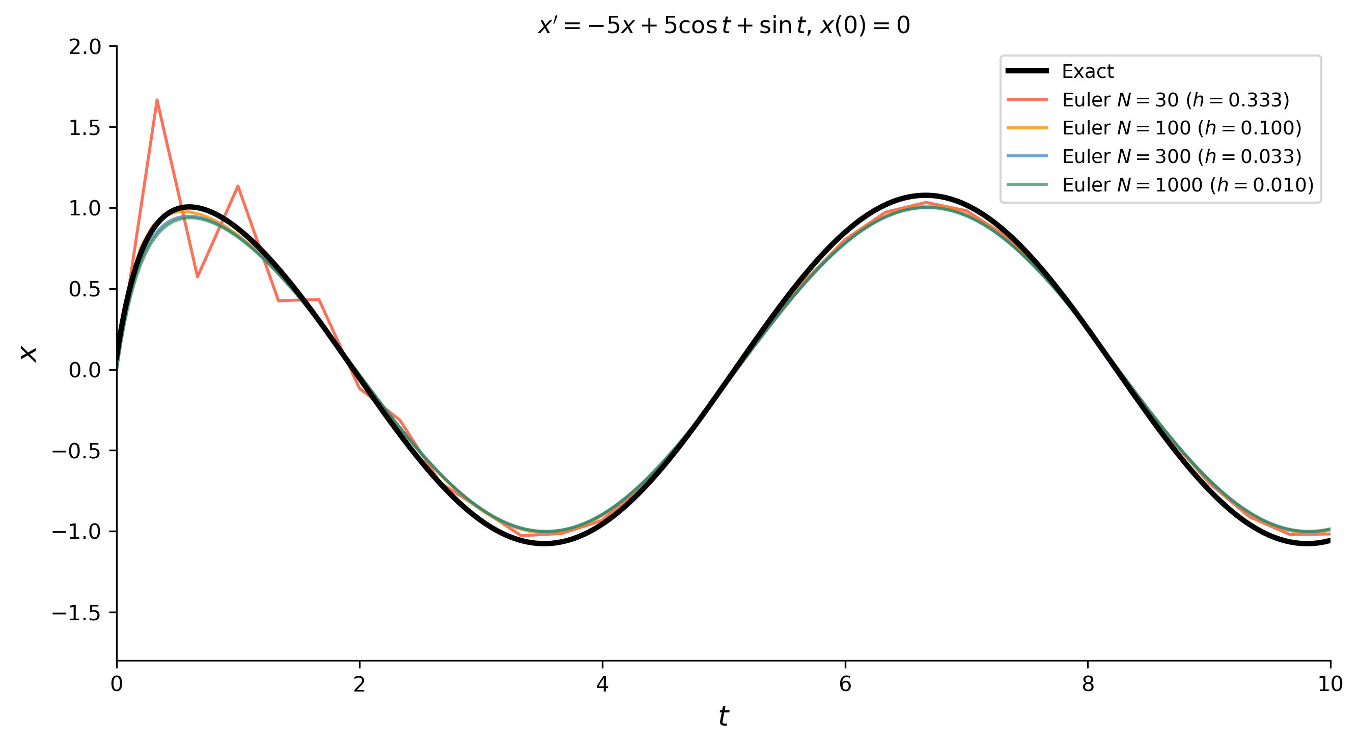
Figure 5: Example 5. Left: rabbit and fox populations over time showing characteristic out-of-phase oscillations. Right: phase portrait (orbit in the \(x\)\(y\) plane) showing the closed trajectory around the coexistence equilibrium \((8,5)\) (green dot).

Example 6 — Second-Order Equation as a System: Damped Nonlinear Pendulum

A damped pendulum satisfies \[ \theta'' + 0.3\,\theta' + \sin\theta = 0, \qquad \theta(0) = \frac{2\pi}{3}, \quad \theta'(0) = 0, \] where \(\theta\) is the angle from the downward vertical (radians) and \(t\) is in seconds.

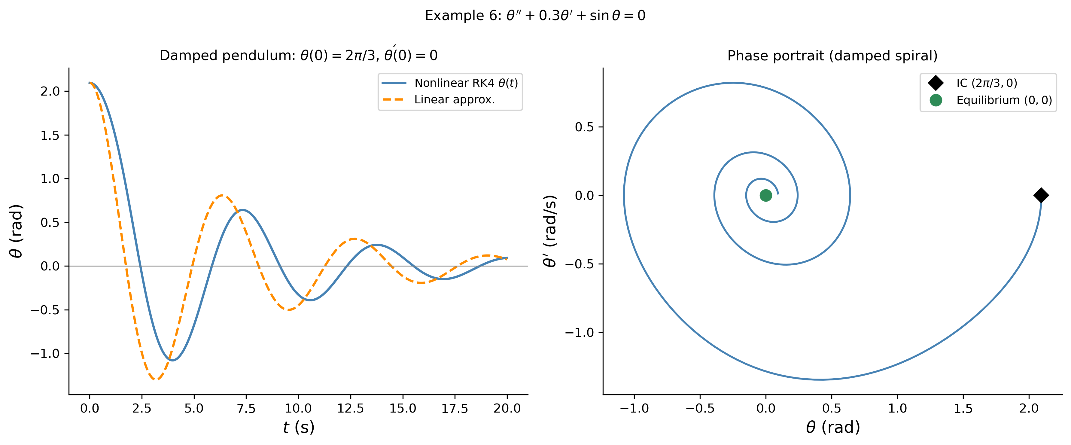
(a) Convert to a first-order system. (b) Use RK4 with \(h = 0.05\) to solve for \(0 \le t \le 20\). (c) Compare with the linearised small-angle approximation to comment on the effect of the large initial angle.

Conversion to a System

Set \(x = \theta\) (angle) and \(y = \theta'\) (angular velocity):

\[ x' = y, \qquad y' = -0.3y - \sin x. \]

Initial conditions: \(x(0) = 2\pi/3 \approx 2.094\), \(y(0) = 0\).

Linearised Approximation

For small \(\theta\): \(\sin\theta \approx \theta\). The linearised equation is \(\theta'' + 0.3\theta' + \theta = 0\), a damped harmonic oscillator with characteristic roots

\[ \lambda = \frac{-0.3 \pm \sqrt{0.09 - 4}}{2} = -0.15 \pm i\sqrt{0.9775}. \]

Quasi-frequency \(\omega_d = \sqrt{0.9775} \approx 0.9887\) rad/s, quasi-period \(T_d = 2\pi/\omega_d \approx 6.35\) s. The general solution is

\[ \theta_{\rm lin}(t) = e^{-0.15t}\!\left(A\cos(\omega_d t) + B\sin(\omega_d t)\right). \]

Applying \(\theta(0) = 2\pi/3\), \(\theta'(0) = 0\): \(A = 2\pi/3\) and \(B = 0.15A/\omega_d = 0.3204\).

Show the code
f6 = lambda t, x, y: y
g6 = lambda t, x, y: -0.3*y - np.sin(x)

x0_6 = 2*np.pi/3
ts6, Xs6, Ys6 = rk4_system(f6, g6, 0.0, x0_6, 0.0, 20.0, h=0.05)

# Linearised solution
omega_d = np.sqrt(1 - 0.15**2)
A = x0_6
B = 0.15*A / omega_d
t_lin = np.linspace(0, 20, 800)
theta_lin = np.exp(-0.15*t_lin) * (A*np.cos(omega_d*t_lin) + B*np.sin(omega_d*t_lin))

fig, axes = plt.subplots(1, 2, figsize=(12, 5))

ax = axes[0]
ax.plot(ts6, Xs6, color='steelblue',  lw=1.8, label=r'Nonlinear RK4 $\theta(t)$')
ax.plot(t_lin, theta_lin, '--', color='darkorange', lw=1.8,
        label='Linear approx.')
ax.axhline(0, color='gray', lw=0.7)
ax.set_xlabel(r'$t$ (s)', fontsize=13)
ax.set_ylabel(r'$\theta$ (rad)', fontsize=13)
ax.set_title(r'Damped pendulum: $\theta(0)=2\pi/3$, $\theta\'(0)=0$', fontsize=11)
ax.legend(fontsize=9)

ax = axes[1]
ax.plot(Xs6, Ys6, color='steelblue', lw=1.5)
ax.plot(x0_6, 0, 'D', color='black',   ms=8, zorder=5,
        label=r'IC $(2\pi/3, 0)$')
ax.plot(0,    0, 'o', color='seagreen', ms=9, zorder=6,
        label='Equilibrium $(0,0)$')
ax.set_xlabel(r'$\theta$ (rad)', fontsize=13)
ax.set_ylabel(r"$\theta'$ (rad/s)", fontsize=13)
ax.set_title('Phase portrait (damped spiral)', fontsize=11)
ax.legend(fontsize=9)

plt.suptitle(r"Example 6: $\theta''+0.3\theta'+\sin\theta=0$", fontsize=11)
plt.tight_layout()
plt.show()
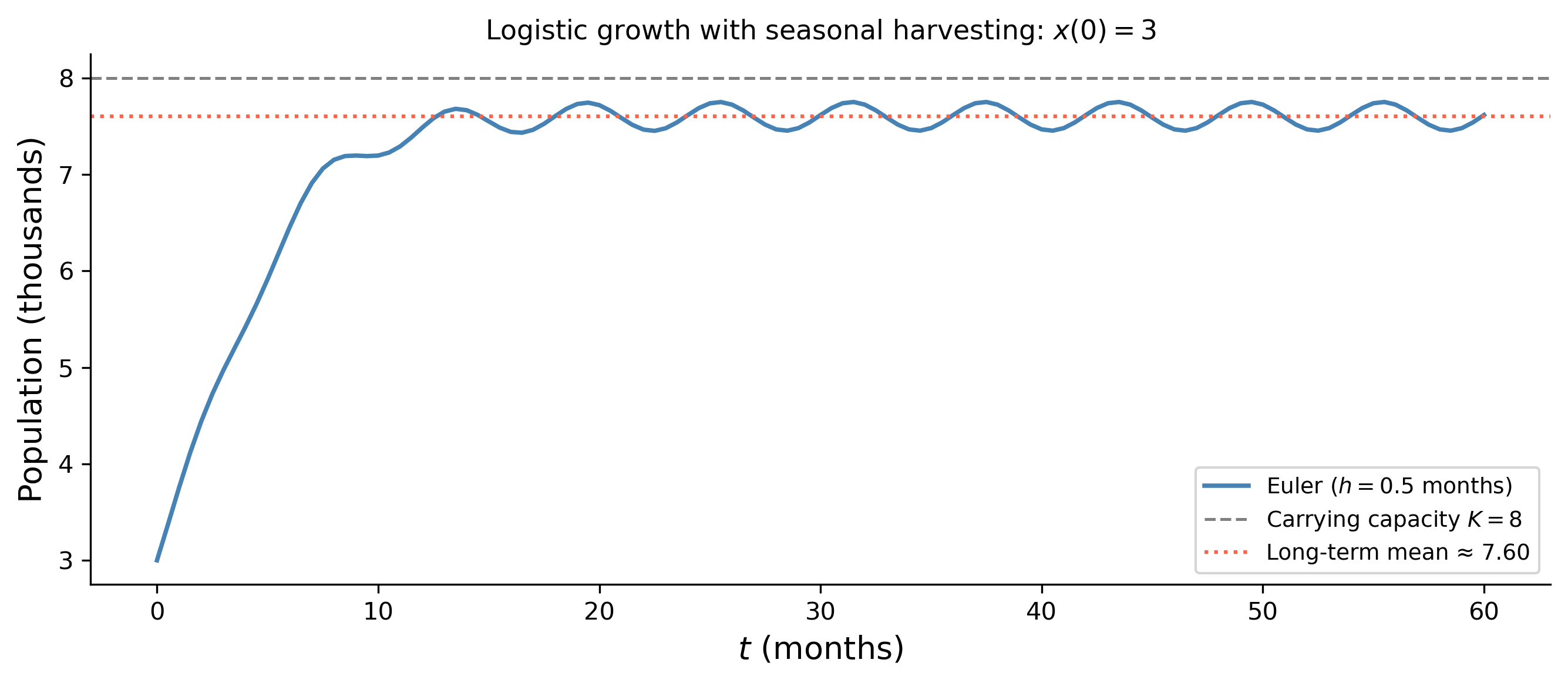
Figure 6: Example 6. Left: RK4 solution for \(\theta(t)\) (steelblue) compared to the small-angle linearisation (dashed orange). The large initial angle \(2\pi/3 \approx 120°\) causes the period of the nonlinear system to differ noticeably from the linear prediction. Right: phase portrait showing the damped spiral converging to the equilibrium at the origin.
Tip

Effect of large amplitude on the period. For the nonlinear pendulum, the period of oscillation increases with amplitude (unlike the hardening spring in §5.2). The exact period at angle \(\Theta_0\) is given by an elliptic integral; for \(\Theta_0 = 120°\) the true period is about \(8.0\) s — roughly \(26\%\) longer than the small-angle period of \(6.35\) s. The linear approximation therefore underestimates the period and gets progressively more out of phase with the nonlinear solution over time, as the figure shows.


Example 7 — RLC Circuit as a System

An RLC circuit has \(R = 2\;\Omega\), \(L = 1\;\text{H}\), \(C = 0.25\;\text{F}\), and a time-varying voltage source \(V(t) = 4e^{-t}\cos 2t\). The charge \(q(t)\) on the capacitor satisfies \[ q'' + 2q' + 4q = 4e^{-t}\cos 2t, \qquad q(0) = 0, \quad q'(0) = 0. \]

(a) Write as a first-order system. (b) Solve using RK4 with \(h = 0.05\) on \([0, 10]\). (c) Plot \(q(t)\) and the current \(I(t) = q'(t)\), and describe the long-term behaviour.

System Formulation

Set \(x = q\) (charge) and \(y = q' = I\) (current):

\[ x' = y, \qquad y' = -4x - 2y + 4e^{-t}\cos 2t. \]

Characteristic Roots and Transient

The homogeneous equation \(q'' + 2q' + 4q = 0\) has characteristic roots

\[ \lambda = \frac{-2 \pm \sqrt{4 - 16}}{2} = -1 \pm i\sqrt{3}. \]

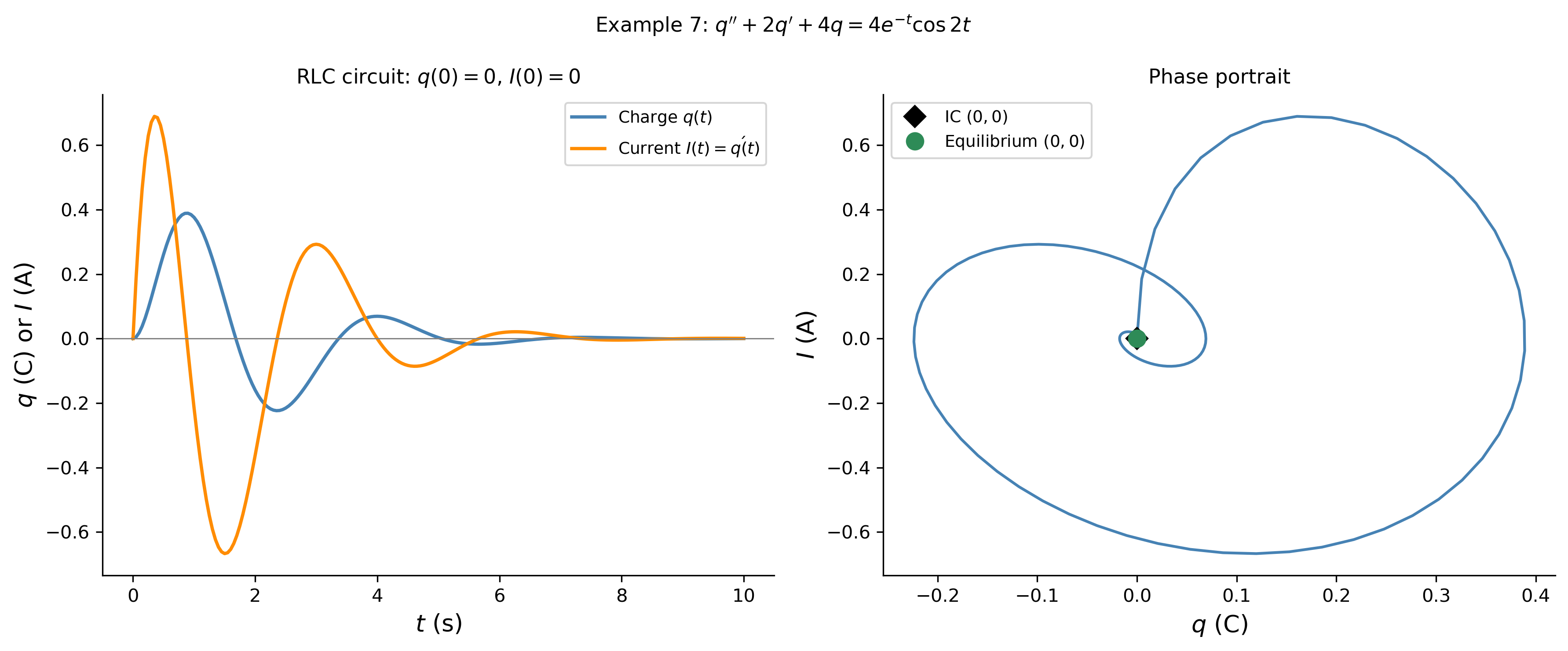
The homogeneous (transient) solution decays like \(e^{-t}\), with quasi-period \(T_d = 2\pi/\sqrt{3} \approx 3.63\) s. Because the forcing \(4e^{-t}\cos 2t\) also decays, the entire response eventually dies out — there is no persistent oscillation here, unlike a sinusoidal forcing.

Show the code
f7 = lambda t, x, y: y
g7 = lambda t, x, y: -4*x - 2*y + 4*np.exp(-t)*np.cos(2*t)

ts7, Xs7, Ys7 = rk4_system(f7, g7, 0.0, 0.0, 0.0, 10.0, h=0.05)

fig, axes = plt.subplots(1, 2, figsize=(12, 5))

ax = axes[0]
ax.plot(ts7, Xs7, color='steelblue',  lw=1.8, label=r'Charge $q(t)$')
ax.plot(ts7, Ys7, color='darkorange', lw=1.8, label=r'Current $I(t)=q\'(t)$')
ax.axhline(0, color='gray', lw=0.7)
ax.set_xlabel(r'$t$ (s)', fontsize=13)
ax.set_ylabel(r'$q$ (C) or $I$ (A)', fontsize=13)
ax.set_title(r'RLC circuit: $q(0)=0$, $I(0)=0$', fontsize=11)
ax.legend(fontsize=9)

ax = axes[1]
ax.plot(Xs7, Ys7, color='steelblue', lw=1.5)
ax.plot(Xs7[0], Ys7[0], 'D', color='black',   ms=8, zorder=5, label='IC $(0,0)$')
ax.plot(0,      0,       'o', color='seagreen', ms=9, zorder=6,
        label='Equilibrium $(0,0)$')
ax.set_xlabel(r'$q$ (C)', fontsize=13)
ax.set_ylabel(r'$I$ (A)', fontsize=13)
ax.set_title('Phase portrait', fontsize=11)
ax.legend(fontsize=9)

plt.suptitle(r"Example 7: $q''+2q'+4q=4e^{-t}\cos2t$", fontsize=11)
plt.tight_layout()
plt.show()
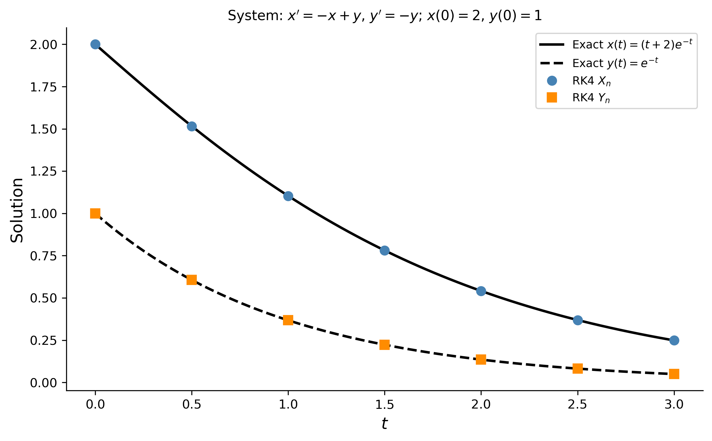
Figure 7: Example 7. Left: charge \(q(t)\) (steelblue) and current \(I(t)=q'(t)\) (orange) versus time. The circuit response peaks around \(t\approx1\)\(2\) s and then decays to zero as both the transient solution and the forcing decay exponentially. Right: phase portrait of \((q, I)\) showing an inward spiral that terminates at the origin.

Example 8 — Accuracy Comparison on a Nonlinear System

For the nonlinear system \[ x' = y - x^2, \qquad y' = -x, \qquad x(0) = 0, \quad y(0) = 1, \] there is no closed-form solution. Use a high-accuracy SciPy reference (solve_ivp with RK45 and tight tolerances) to compare the Euler, modified Euler, and RK4 methods at \(t = 3\) for step sizes \(h = 0.5, 0.25, 0.1, 0.05\).

from scipy.integrate import solve_ivp as sp_ivp

def sys8_scipy(t, s):
    x, y = s
    return [y - x**2, -x]

ref = sp_ivp(sys8_scipy, [0, 3], [0.0, 1.0],
             method='RK45', rtol=1e-11, atol=1e-13, dense_output=True)
x_ref, y_ref = ref.sol(3.0)
print(f"High-accuracy reference: x(3) ≈ {x_ref:.10f},  y(3) ≈ {y_ref:.10f}")
High-accuracy reference: x(3) ≈ 0.1557851166,  y(3) ≈ -0.3809790629
def euler_system(f, g, t0, x0, y0, T, h):
    """Euler method for 2x2 system."""
    t, x, y = t0, x0, y0
    while t < T - 1e-12:
        xn = x + h*f(t, x, y)
        yn = y + h*g(t, x, y)
        x, y, t = xn, yn, t + h
    return x, y

def heun_system(f, g, t0, x0, y0, T, h):
    """Modified Euler (Heun) for 2x2 system."""
    t, x, y = t0, x0, y0
    while t < T - 1e-12:
        k1x = f(t, x, y);      k1y = g(t, x, y)
        k2x = f(t+h, x+h*k1x, y+h*k1y)
        k2y = g(t+h, x+h*k1x, y+h*k1y)
        x = x + h/2*(k1x + k2x)
        y = y + h/2*(k1y + k2y)
        t += h
    return x, y

f8 = lambda t, x, y: y - x**2
g8 = lambda t, x, y: -x
T8 = 3.0

print(f"{'h':>6}  {'Euler |err_x|':>15}  {'Heun |err_x|':>14}  {'RK4 |err_x|':>13}")
print("-" * 55)
for h in [0.5, 0.25, 0.1, 0.05]:
    xe, ye   = euler_system(f8, g8, 0, 0, 1, T8, h)
    xm, ym   = heun_system(f8, g8, 0, 0, 1, T8, h)
    _, Xrk, _ = rk4_system(f8, g8, 0.0, 0.0, 1.0, T8, h)
    Xrk_T = Xrk[-1]
    print(f"{h:>6.2f}  {abs(xe-x_ref):>15.2e}  {abs(xm-x_ref):>14.2e}  {abs(Xrk_T-x_ref):>13.2e}")
     h    Euler |err_x|    Heun |err_x|    RK4 |err_x|
-------------------------------------------------------
  0.50         7.21e-02        4.03e-02       3.56e-04
  0.25         3.84e-02        9.13e-03       1.81e-05
  0.10         1.55e-02        1.35e-03       4.14e-07
  0.05         7.74e-03        3.28e-04       2.50e-08
Show the code
hs8 = np.array([0.5, 0.25, 0.1, 0.05, 0.025])
err_e8 = []; err_m8 = []; err_rk8 = []
for h in hs8:
    xe, _  = euler_system(f8, g8, 0, 0, 1, T8, h)
    xm, _  = heun_system(f8, g8, 0, 0, 1, T8, h)
    _, Xrk, _ = rk4_system(f8, g8, 0.0, 0.0, 1.0, T8, h)
    err_e8.append(abs(xe - x_ref))
    err_m8.append(abs(xm - x_ref))
    err_rk8.append(abs(Xrk[-1] - x_ref))

fig, axes = plt.subplots(1, 2, figsize=(12, 5))

ax = axes[0]
ax.loglog(hs8, err_e8,  'o-', color='tomato',    lw=1.8, ms=7, label='Euler')
ax.loglog(hs8, err_m8,  's-', color='darkorange', lw=1.8, ms=7, label='Mod. Euler')
ax.loglog(hs8, err_rk8, '^-', color='steelblue',  lw=1.8, ms=7, label='RK4')
ax.loglog(hs8, 2.0*hs8,       'k:',  lw=1.2, label=r'$O(h)$')
ax.loglog(hs8, 1.5*hs8**2,    'k--', lw=1.2, label=r'$O(h^2)$')
ax.loglog(hs8, 0.8*hs8**4,    'k-.', lw=1.2, label=r'$O(h^4)$')
ax.set_xlabel(r'Step size $h$', fontsize=13)
ax.set_ylabel(r'$|X_N - x_{\rm ref}(3)|$', fontsize=13)
ax.set_title('Error in $x(3)$ for the nonlinear system', fontsize=11)
ax.legend(fontsize=8)

ax = axes[1]
t_dense = np.linspace(0, T8, 500)
xy_dense = ref.sol(t_dense)
ax.plot(xy_dense[0], xy_dense[1], color='steelblue', lw=1.8)
ax.plot(0, 1, 'D', color='black',   ms=8, zorder=5, label='IC $(0,1)$')
ax.set_xlabel(r'$x$', fontsize=13)
ax.set_ylabel(r'$y$', fontsize=13)
ax.set_title('Reference phase portrait', fontsize=11)
ax.legend(fontsize=9)

plt.suptitle(r"Example 8: $x'=y-x^2$, $y'=-x$", fontsize=11)
plt.tight_layout()
plt.show()
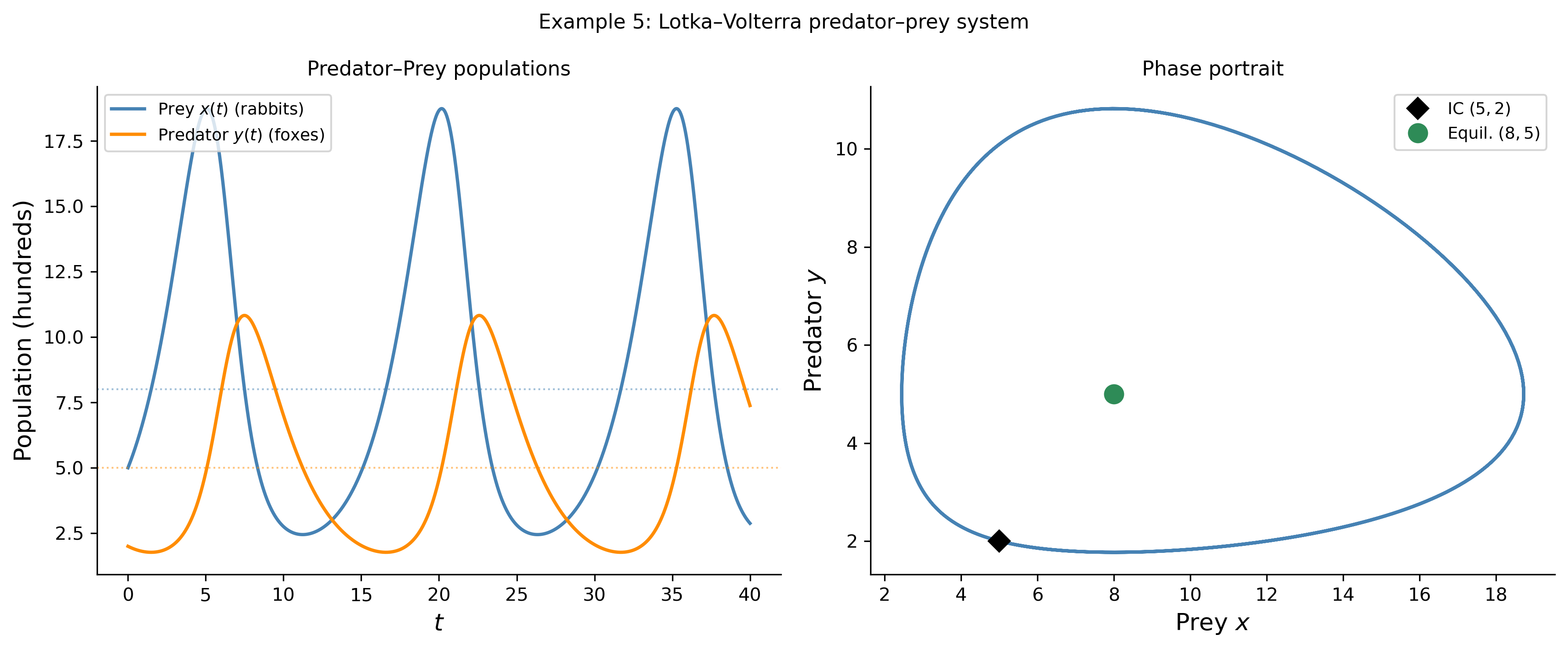
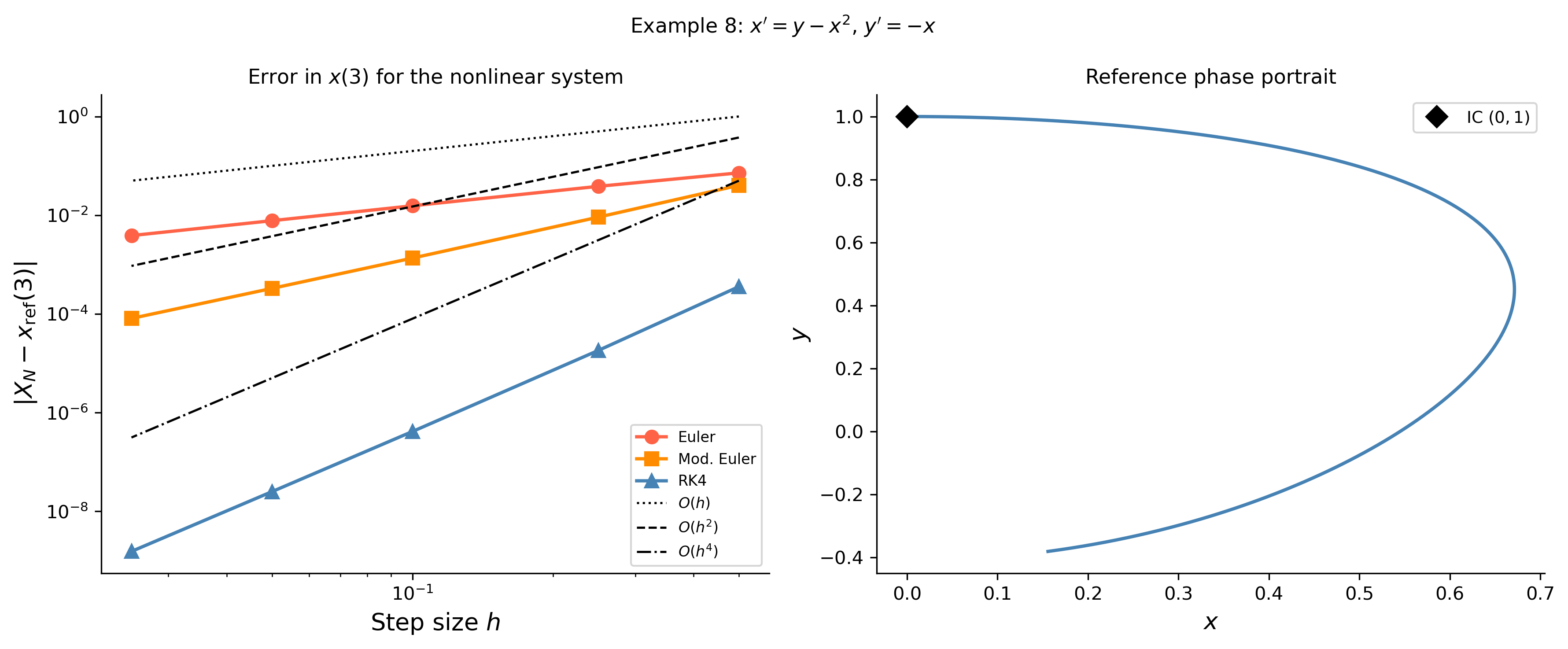
Figure 8: Example 8. Left: log–log error plot for \(x(3)\) confirming \(O(h)\), \(O(h^2)\), and \(O(h^4)\) convergence on the nonlinear system. Right: phase portrait showing the trajectory from \((0,1)\) computed by the high-accuracy reference solver.
Note

Summary of method orders. Across all examples in this document, the error tables confirm the theoretical convergence rates: halving \(h\) reduces the Euler error by roughly \(2\times\), the modified Euler error by \(4\times\), and the RK4 error by \(16\times\). For the nonlinear system in Example 8 the same rates hold, showing that the order of accuracy is a property of the method, not of the specific equation.


References

Logan, J David. 2015. A First Course in Differential Equations, Third Edition.
import sys
print("Python version:", sys.version)
print('\n'.join(f'{m.__name__}=={m.__version__}'
                for m in globals().values()
                if getattr(m, '__version__', None)))
Python version: 3.14.4 | packaged by conda-forge | (main, Apr  8 2026, 02:33:53) [Clang 20.1.8 ]
numpy==2.4.3
sympy==1.14.0
matplotlib==3.10.8

Reuse

CC BY-NC-SA 4.0