First-Order Equations — Worked Examples

Show the code

# This is a code cell that imports the necessary libraries for our session.
import numpy as np                        # NumPy for numerical computations
import sympy as sym                       # SymPy for symbolic mathematics
import matplotlib as mpl                  # Matplotlib for plotting
import matplotlib.pyplot as plt           # Matplotlib pyplot interface
from IPython.display import Math, display
mpl.rcParams['figure.dpi'] = 150
mpl.rcParams['axes.spines.top'] = False
mpl.rcParams['axes.spines.right'] = False

In this document we work through fully solved examples corresponding to the topics in Homework 2: sketching slope fields (§1.1.3), solving separable equations (§1.3.1), solving first-order linear equations via integrating factors (§1.4.1), and applications to mechanics, population biology, and electric circuits (§1.4.3).

Example 1 — Sketching a Slope Field

Sketch the slope field for the differential equation \[\frac{dy}{dx} = y - x,\] and identify the qualitative behavior of solutions.

By Hand

A slope field (also called a direction field) is a picture of the right-hand side $f(x, y)$ of the equation $y' = f(x,y)$: at each point $(x, y)$ in the plane we draw a short line segment whose slope equals $f(x, y) = y - x$.

Step 1 — Build a table of representative slopes.

It is helpful to first find the isoclines, curves along which the slope is constant. Setting $y - x = c$ gives the family of lines $y = x + c$. Along each such line every slope segment has the same slope $c$.

Isocline $y = x + c$	Slope of segments
$y = x - 2$	$-2$
$y = x - 1$	$-1$
$y = x$	$0$ (horizontal segments)
$y = x + 1$	$1$
$y = x + 2$	$2$

The isocline $y = x$ (i.e. $c = 0$) is where the slope segments are horizontal.

Step 2 — Draw the segments.

Starting from the $c = 0$ isocline $y = x$, draw horizontal segments. Moving above this line (larger $y - x$) the slopes become increasingly positive; moving below it the slopes become increasingly negative.

Step 3 — Sketch solution curves.

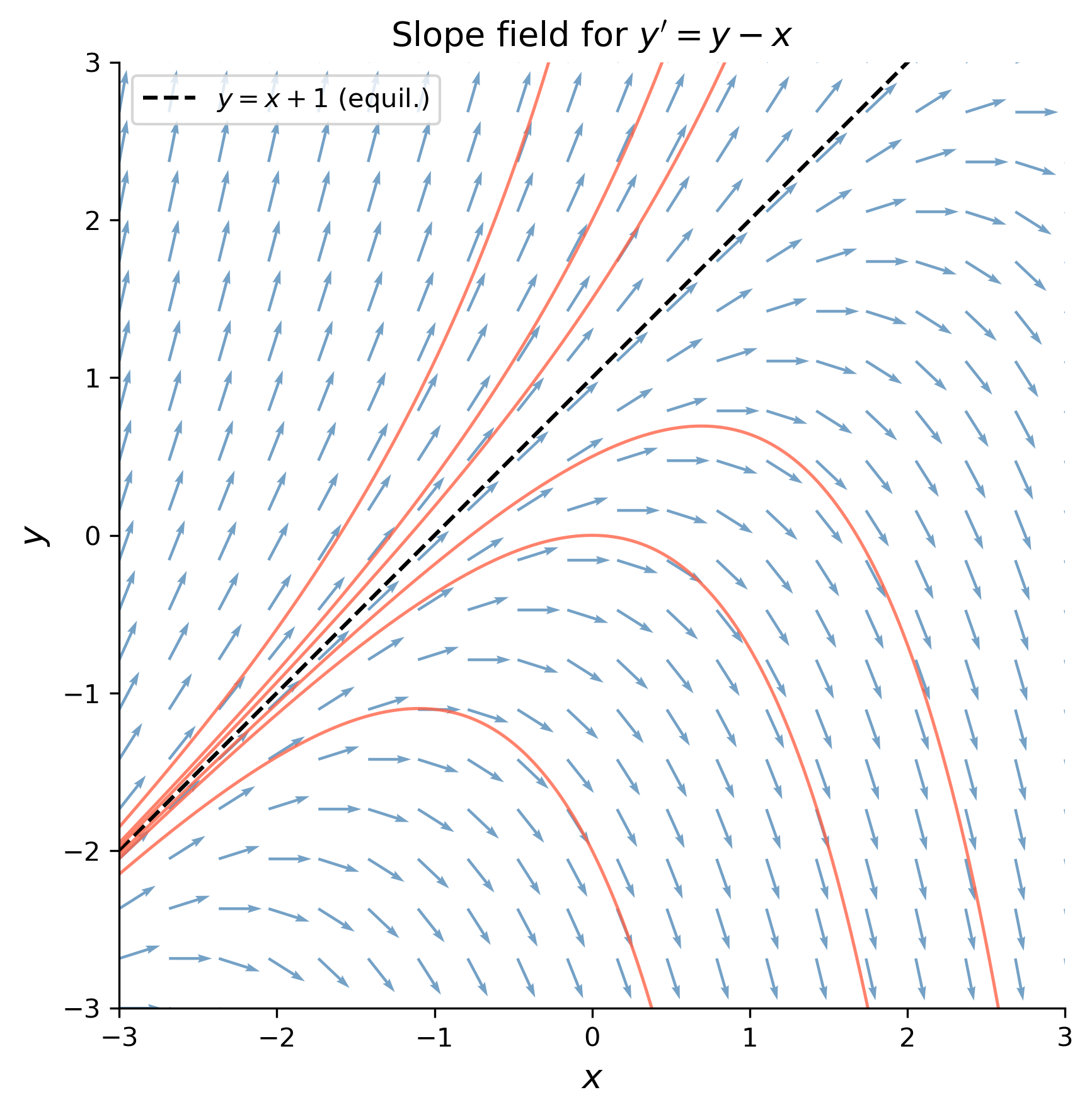
Tracing along the slope segments suggests that solutions are attracted toward the line $y = x + 1$. We can confirm this analytically: the general solution (found in Example 3 below) is $y(x) = Ce^{x} + x + 1$, which for any finite $C$ satisfies $y(x) - (x+1) = Ce^x \to \pm\infty$ as $x \to \infty$ (not bounded toward the line for $C \neq 0$). However, the particular solution $C = 0$ is exactly $y = x + 1$, the unique equilibrium line (straight-line solution) of this equation.

Tip

Isocline strategy. To sketch a slope field quickly, find the isoclines $f(x,y) = c$ for several values of $c$, draw the corresponding line-segment slopes along each isocline, then sketch a few representative solution curves by “following the flow.”

Using SymPy

We use SymPy to generate a fine grid of slope segments and plot the field.

Show the code

x_vals = np.linspace(-3, 3, 20)
y_vals = np.linspace(-3, 3, 20)
X, Y = np.meshgrid(x_vals, y_vals)

# Right-hand side: f(x,y) = y - x
dY = Y - X
dX = np.ones_like(dY)

# Normalise for uniform arrow length
length = np.sqrt(dX**2 + dY**2)
dX_n = dX / length
dY_n = dY / length

fig, ax = plt.subplots(figsize=(6, 6))
ax.quiver(X, Y, dX_n, dY_n,
          angles='xy', scale=22, width=0.003,
          color='steelblue', alpha=0.75)

# Equilibrium line y = x + 1
x_line = np.linspace(-3, 3, 200)
ax.plot(x_line, x_line + 1, 'k--', lw=1.5, label=r'$y = x + 1$ (equil.)')

# A few representative solution curves  y = C e^x + x + 1
for C in [-3, -1, -0.5, 0.5, 1, 3]:
    y_sol = C * np.exp(x_line) + x_line + 1
    mask = np.abs(y_sol) < 4
    ax.plot(x_line[mask], y_sol[mask], color='tomato', lw=1.2, alpha=0.8)

ax.set_xlim(-3, 3)
ax.set_ylim(-3, 3)
ax.set_xlabel(r'$x$', fontsize=13)
ax.set_ylabel(r'$y$', fontsize=13)
ax.set_title(r"Slope field for $y' = y - x$", fontsize=13)
ax.legend(fontsize=10)
ax.set_aspect('equal')
plt.tight_layout()
plt.show()

Figure 1: Slope field for $y' = y - x$. The dashed line $y = x+1$ is the equilibrium (straight-line) solution $y = x+1$.

Example 2 — Solving a Separable Equation

Find the general solution of the separable equation \[\frac{dy}{dx} = \frac{x^2}{1 - y^2},\] and solve the initial value problem with $y(0) = 0$.

By Hand

Step 1 — Separate variables.

Rewrite the equation so that all $y$-terms are on the left and all $x$-terms are on the right: \[ (1 - y^2)\,dy = x^2\,dx. \]

Step 2 — Integrate both sides.

\[ \int (1 - y^2)\,dy = \int x^2\,dx \quad\Longrightarrow\quad y - \frac{y^3}{3} = \frac{x^3}{3} + C, \]

where $C$ is an arbitrary constant of integration.

Step 3 — State the general (implicit) solution.

\[ \boxed{y - \frac{y^3}{3} = \frac{x^3}{3} + C.} \]

Because we cannot solve this cubic in $y$ in a simple closed form, we leave the solution in implicit form.

Step 4 — Apply the initial condition $y(0) = 0$.

Substitute $x = 0$, $y = 0$: \[ 0 - \frac{0}{3} = \frac{0}{3} + C \quad\Longrightarrow\quad C = 0. \]

The particular solution satisfying the initial condition is \[ \boxed{y - \frac{y^3}{3} = \frac{x^3}{3}.} \]

Multiplying through by $3$ gives the equivalent form $3y - y^3 = x^3$.

Note

The separation of variables method requires that $1 - y^2 \neq 0$, i.e. $y \neq \pm 1$. These correspond to the constant (equilibrium) solutions $y = 1$ and $y = -1$, which can be verified by direct substitution: if $y = \pm 1$ then $dy/dx = 0$ and $x^2/(1-1) $ is undefined, so in fact neither $y = 1$ nor $y = -1$ is a solution. The restriction $y \neq \pm 1$ is needed to perform the separation, but these values simply lie outside the domain of the equation as written.

Using SymPy

x = sym.Symbol('x')
y = sym.Function('y')   # y must be a Function, not a Symbol, for dsolve

# Define the ODE   dy/dx = x^2 / (1 - y^2)
ode = sym.Eq(y(x).diff(x), x**2 / (1 - y(x)**2))

# SymPy's dsolve handles separable equations
sol = sym.dsolve(ode, y(x))
display(Math(r'\text{General solution: }' + sym.latex(sol)))

\(\displaystyle \text{General solution: }\left[ y{\left(x \right)} = \sqrt[3]{2} \left(\frac{\sqrt[3]{2} \sqrt[3]{- 3 C_{1} + x^{3} + \sqrt{9 C_{1}^{2} - 6 C_{1} x^{3} + x^{6} - 4}}}{4} + \frac{\sqrt[3]{2} \sqrt{3} i \sqrt[3]{- 3 C_{1} + x^{3} + \sqrt{9 C_{1}^{2} - 6 C_{1} x^{3} + x^{6} - 4}}}{4} - \frac{2}{\left(-1 - \sqrt{3} i\right) \sqrt[3]{- 3 C_{1} + x^{3} + \sqrt{9 C_{1}^{2} - 6 C_{1} x^{3} + x^{6} - 4}}}\right), \ y{\left(x \right)} = \sqrt[3]{2} \left(\frac{\sqrt[3]{2} \sqrt[3]{- 3 C_{1} + x^{3} + \sqrt{9 C_{1}^{2} - 6 C_{1} x^{3} + x^{6} - 4}}}{4} - \frac{\sqrt[3]{2} \sqrt{3} i \sqrt[3]{- 3 C_{1} + x^{3} + \sqrt{9 C_{1}^{2} - 6 C_{1} x^{3} + x^{6} - 4}}}{4} - \frac{2}{\left(-1 + \sqrt{3} i\right) \sqrt[3]{- 3 C_{1} + x^{3} + \sqrt{9 C_{1}^{2} - 6 C_{1} x^{3} + x^{6} - 4}}}\right), \ y{\left(x \right)} = \sqrt[3]{2} \left(- \frac{\sqrt[3]{2} \sqrt[3]{- 3 C_{1} + x^{3} + \sqrt{9 C_{1}^{2} - 6 C_{1} x^{3} + x^{6} - 4}}}{2} - \frac{1}{\sqrt[3]{- 3 C_{1} + x^{3} + \sqrt{9 C_{1}^{2} - 6 C_{1} x^{3} + x^{6} - 4}}}\right)\right]\)

# Apply the initial condition y(0) = 0
sol_ivp = sym.dsolve(ode, y(x), ics={y(0): 0})
display(Math(r'\text{Particular solution: }' + sym.latex(sol_ivp)))

$\displaystyle \text{Particular solution: }y{\left(x \right)} = \sqrt[3]{2} \left(\frac{\sqrt[3]{2} \sqrt[3]{x^{3} + \sqrt{x^{6} - 4}}}{4} + \frac{\sqrt[3]{2} \sqrt{3} i \sqrt[3]{x^{3} + \sqrt{x^{6} - 4}}}{4} - \frac{2}{\left(-1 - \sqrt{3} i\right) \sqrt[3]{x^{3} + \sqrt{x^{6} - 4}}}\right)$

Note

SymPy returns the solution in explicit form when it can invert the implicit relation; for this cubic it expresses the answer using the real cube root. The by-hand implicit form $y - y^3/3 = x^3/3$ and the SymPy result are equivalent.

Example 3 — Solving a First-Order Linear Equation (Integrating Factor)

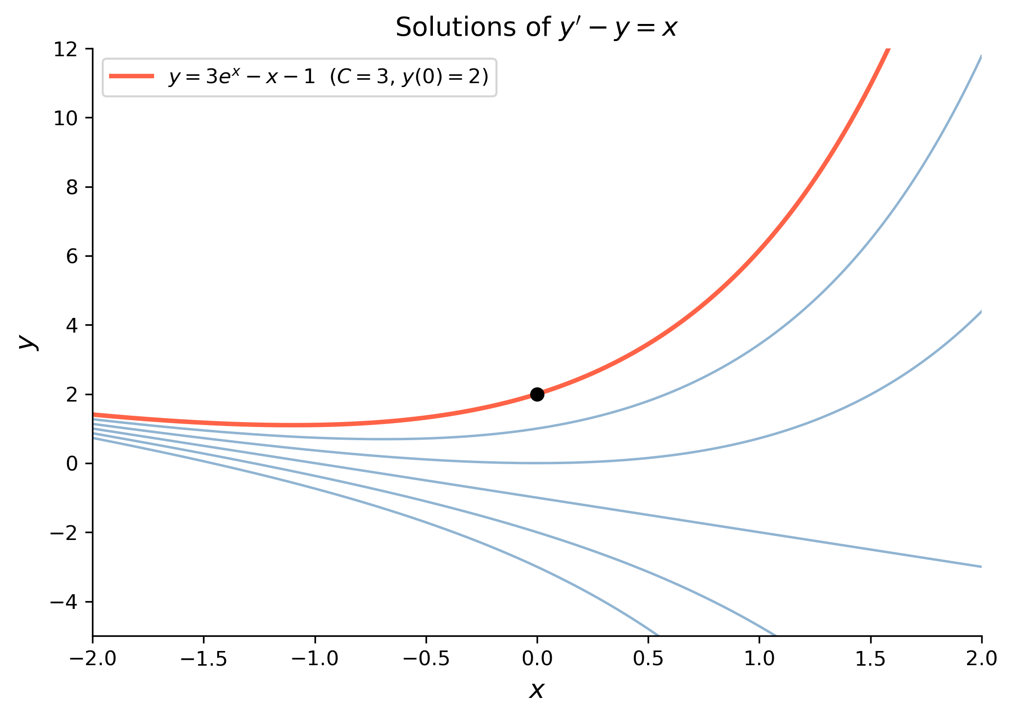
Solve the initial value problem \[\frac{dy}{dx} - y = x, \qquad y(0) = 2.\]

By Hand

A first-order linear ODE has the standard form \[ \frac{dy}{dx} + P(x)\,y = Q(x). \]

Here $P(x) = -1$ and $Q(x) = x$.

Step 1 — Compute the integrating factor.

\[ \mu(x) = e^{\int P(x)\,dx} = e^{\int (-1)\,dx} = e^{-x}. \]

Step 2 — Multiply both sides by $\mu(x) = e^{-x}$.

\[ e^{-x}\frac{dy}{dx} - e^{-x} y = x e^{-x}. \]

The left-hand side is now the derivative of the product $\mu(x) y$: \[ \frac{d}{dx}\!\left[e^{-x} y\right] = x e^{-x}. \]

Step 3 — Integrate both sides.

\[ e^{-x} y = \int x e^{-x}\,dx. \]

Use integration by parts with $u = x$, $dv = e^{-x}\,dx$: \[ \int x e^{-x}\,dx = -x e^{-x} - \int (-e^{-x})\,dx = -x e^{-x} - e^{-x} + C = -(x+1)e^{-x} + C. \]

Therefore \[ e^{-x} y = -(x+1)e^{-x} + C. \]

Step 4 — Solve for $y$.

Divide through by $e^{-x}$ (equivalently, multiply by $e^x$): \[ y = -(x+1) + Ce^{x} = Ce^{x} - x - 1. \]

The general solution is \[ \boxed{y(x) = Ce^{x} - x - 1.} \]

Step 5 — Apply the initial condition $y(0) = 2$.

\[ y(0) = C e^{0} - 0 - 1 = C - 1 = 2 \quad\Longrightarrow\quad C = 3. \]

The particular solution is \[ \boxed{y(x) = 3e^{x} - x - 1.} \]

Verification. Differentiate: $y'(x) = 3e^x - 1$. Check $y' - y$: \[ (3e^x - 1) - (3e^x - x - 1) = 3e^x - 1 - 3e^x + x + 1 = x. \checkmark \]

And $y(0) = 3(1) - 0 - 1 = 2$. $\checkmark$

Using SymPy

x = sym.Symbol('x')
y = sym.Function('y')

ode3 = sym.Eq(y(x).diff(x) - y(x), x)

# General solution
gen_sol = sym.dsolve(ode3, y(x))
display(Math(r'\text{General solution: } ' + sym.latex(gen_sol)))

# Particular solution with y(0) = 2
part_sol = sym.dsolve(ode3, y(x), ics={y(0): 2})
display(Math(r'\text{Particular solution: } ' + sym.latex(part_sol)))

$\displaystyle \text{General solution: } y{\left(x \right)} = C_{1} e^{x} - x - 1$

$\displaystyle \text{Particular solution: } y{\left(x \right)} = - x + 3 e^{x} - 1$

Show the code

x_vals = np.linspace(-2, 2, 400)
fig, ax = plt.subplots(figsize=(7, 5))

for C in [-2, -1, 0, 1, 2]:
    y_sol = C * np.exp(x_vals) - x_vals - 1
    lw = 1.2
    color = 'steelblue'
    ax.plot(x_vals, y_sol, color=color, lw=lw, alpha=0.6)

# Highlight the particular solution C = 3
y_part = 3 * np.exp(x_vals) - x_vals - 1
ax.plot(x_vals, y_part, color='tomato', lw=2.2,
        label=r'$y = 3e^x - x - 1$  ($C=3$, $y(0)=2$)')
ax.plot(0, 2, 'ko', ms=6, zorder=5)

ax.set_xlim(-2, 2)
ax.set_ylim(-5, 12)
ax.set_xlabel(r'$x$', fontsize=13)
ax.set_ylabel(r'$y$', fontsize=13)
ax.set_title(r"Solutions of $y' - y = x$", fontsize=13)
ax.legend(fontsize=10)
plt.tight_layout()
plt.show()

Figure 2: Solution curves of $y' - y = x$ for several values of $C$, with the particular solution $y = 3e^x - x - 1$ (satisfying $y(0)=2$) highlighted in red.

Example 4 — Application: Newton’s Law of Cooling (Mechanics/Physics)

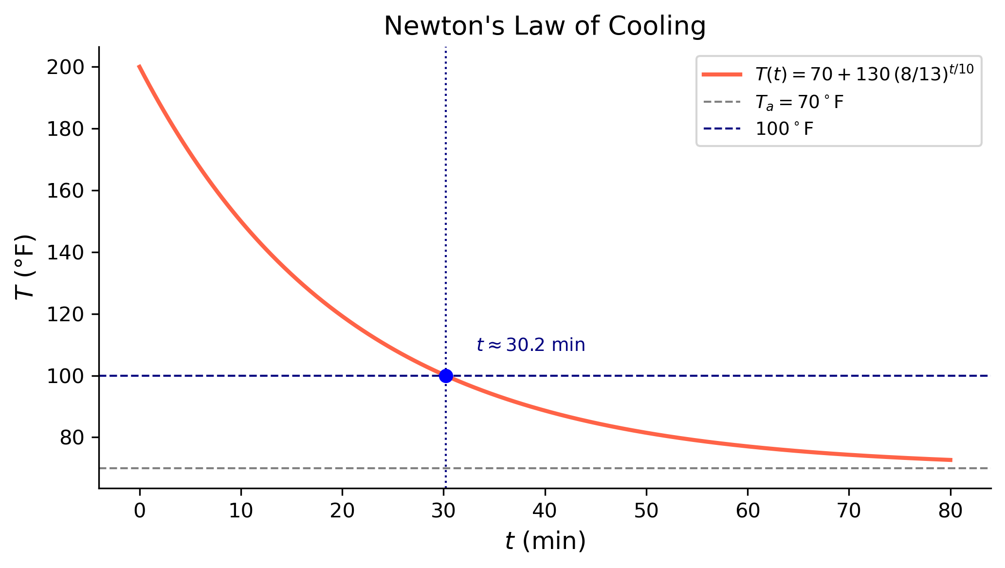
A metal rod is heated to $200^\circ$F and then placed in a room held at a constant temperature of $70^\circ$F. After 10 minutes the temperature of the rod is $150^\circ$F. Find the temperature of the rod as a function of time, and determine how long it takes the rod to reach $100^\circ$F.

By Hand

Newton’s Law of Cooling states that the rate of change of an object’s temperature $T(t)$ is proportional to the difference between the object’s temperature and the ambient (surrounding) temperature $T_a$: \[ \frac{dT}{dt} = -k\bigl(T - T_a\bigr), \qquad k > 0. \]

Here $T_a = 70$ and the initial condition is $T(0) = 200$.

Step 1 — Solve the separable equation.

Separate variables: \[ \frac{dT}{T - 70} = -k\,dt. \] Integrate both sides: \[ \ln|T - 70| = -kt + C_1. \] Exponentiate: \[ T(t) - 70 = Ae^{-kt}, \quad A = \pm e^{C_1}. \] Thus \[ T(t) = 70 + Ae^{-kt}. \]

Step 2 — Apply the initial condition $T(0) = 200$.

\[ 200 = 70 + A e^{0} = 70 + A \quad\Longrightarrow\quad A = 130. \]

So $T(t) = 70 + 130e^{-kt}$.

Step 3 — Use $T(10) = 150$ to find $k$.

\[ 150 = 70 + 130 e^{-10k} \quad\Longrightarrow\quad e^{-10k} = \frac{80}{130} = \frac{8}{13}. \]

Taking the natural logarithm: \[ -10k = \ln\!\left(\frac{8}{13}\right) \quad\Longrightarrow\quad k = -\frac{1}{10}\ln\!\left(\frac{8}{13}\right) = \frac{1}{10}\ln\!\left(\frac{13}{8}\right). \]

Numerically, $k \approx \dfrac{\ln(13/8)}{10} \approx 0.04855$ min$^{-1}$.

The temperature function is \[ \boxed{T(t) = 70 + 130\left(\frac{8}{13}\right)^{t/10}.} \]

Step 4 — Find when $T = 100^\circ$F.

\[ 100 = 70 + 130\left(\frac{8}{13}\right)^{t/10} \quad\Longrightarrow\quad \left(\frac{8}{13}\right)^{t/10} = \frac{30}{130} = \frac{3}{13}. \]

Take the natural logarithm: \[ \frac{t}{10}\ln\!\left(\frac{8}{13}\right) = \ln\!\left(\frac{3}{13}\right) \quad\Longrightarrow\quad t = 10\,\frac{\ln(3/13)}{\ln(8/13)}. \]

Numerically: \[ t = 10\cdot\frac{\ln(3/13)}{\ln(8/13)} = 10\cdot\frac{-1.4663}{-0.4855} \approx 30.2 \text{ minutes}. \]

\[ \boxed{T = 100^\circ\text{F} \text{ is reached after approximately } 30.2 \text{ minutes.}} \]

Using SymPy

t, k = sym.symbols('t k', positive=True)
T    = sym.Function('T')
Ta   = sym.Integer(70)

ode4 = sym.Eq(T(t).diff(t), -k * (T(t) - Ta))

# General solution
gen4 = sym.dsolve(ode4, T(t), ics={T(0): 200})
display(Math(r'T(t) = ' + sym.latex(gen4.rhs)))

# Substitute T(10) = 150 to find k
k_val = sym.solve(gen4.rhs.subs(t, 10) - 150, k)[0]
display(Math(r'k = ' + sym.latex(k_val) + r'\approx ' +
             str(round(float(k_val), 5))))

# Full particular solution
T_sol = gen4.rhs.subs(k, k_val)
display(Math(r'T(t) = ' + sym.latex(sym.simplify(T_sol))))

# Time to reach 100°F
t_star = sym.solve(T_sol - 100, t)[0]
display(Math(r't^* = ' + sym.latex(t_star) +
             r'\approx ' + str(round(float(t_star), 2)) + r'\text{ min}'))

$\displaystyle T(t) = 70 + 130 e^{- k t}$

$\displaystyle k = \log{\left(\frac{\sqrt[10]{13} \cdot 2^{\frac{7}{10}}}{2} \right)}\approx 0.04855$

$\displaystyle T(t) = 70 + 130 \cdot 13^{- \frac{t}{10}} \cdot 2^{\frac{3 t}{10}}$

$\displaystyle t^* = \log{\left(\left(\frac{13}{3}\right)^{\frac{10}{\log{\left(\frac{13}{8} \right)}}} \right)}\approx 30.2\text{ min}$

Show the code

k_num  = float(k_val)
t_star_num = float(t_star)
t_plot = np.linspace(0, 80, 500)
T_plot = 70 + 130 * np.exp(-k_num * t_plot)

fig, ax = plt.subplots(figsize=(7, 4))
ax.plot(t_plot, T_plot, color='tomato', lw=2, label=r'$T(t) = 70 + 130\,(8/13)^{t/10}$')
ax.axhline(70,  color='gray',  ls='--', lw=1, label=r'$T_a = 70^\circ$F')
ax.axhline(100, color='navy',  ls='--', lw=1, label=r'$100^\circ$F')
ax.axvline(t_star_num, color='navy', ls=':', lw=1)
ax.plot(t_star_num, 100, 'bo', ms=6, zorder=5)
ax.annotate(f'$t \\approx {t_star_num:.1f}$ min',
            xy=(t_star_num, 100), xytext=(t_star_num + 3, 108),
            fontsize=9, color='navy')
ax.set_xlabel(r'$t$ (min)', fontsize=12)
ax.set_ylabel(r'$T$ (°F)', fontsize=12)
ax.set_title("Newton's Law of Cooling", fontsize=13)
ax.legend(fontsize=9)
plt.tight_layout()
plt.show()

Figure 3: Temperature of the rod over time according to Newton’s Law of Cooling. The dashed horizontal lines mark the ambient temperature (70°F), the initial temperature (200°F), and the target temperature (100°F).

Example 5 — Application: Population Growth with Harvesting

A fish population in a lake grows at a per-capita rate of $r = 0.4$ per year, but fish are harvested at a constant rate of $H = 500$ fish per year. The initial population is $P(0) = 2000$ fish. Find $P(t)$ and determine whether the population survives long-term.

By Hand

The model is a first-order linear equation: \[ \frac{dP}{dt} = rP - H = 0.4P - 500, \qquad P(0) = 2000. \]

Step 1 — Write in standard linear form.

\[ \frac{dP}{dt} - 0.4P = -500. \]

Here $P(\cdot) = -0.4$ (constant) and $Q(\cdot) = -500$ (constant).

Step 2 — Compute the integrating factor.

\[ \mu(t) = e^{\int (-0.4)\,dt} = e^{-0.4t}. \]

Step 3 — Multiply through and integrate.

\[ \frac{d}{dt}\!\left[e^{-0.4t}P\right] = -500\,e^{-0.4t}. \]

\[ e^{-0.4t}P = \int -500\,e^{-0.4t}\,dt = \frac{-500}{-0.4}\,e^{-0.4t} + C = 1250\,e^{-0.4t} + C. \]

Step 4 — Solve for $P$.

\[ P(t) = 1250 + Ce^{0.4t}. \]

Step 5 — Apply $P(0) = 2000$.

\[ 2000 = 1250 + C \quad\Longrightarrow\quad C = 750. \]

The particular solution is \[ \boxed{P(t) = 1250 + 750\,e^{0.4t}.} \]

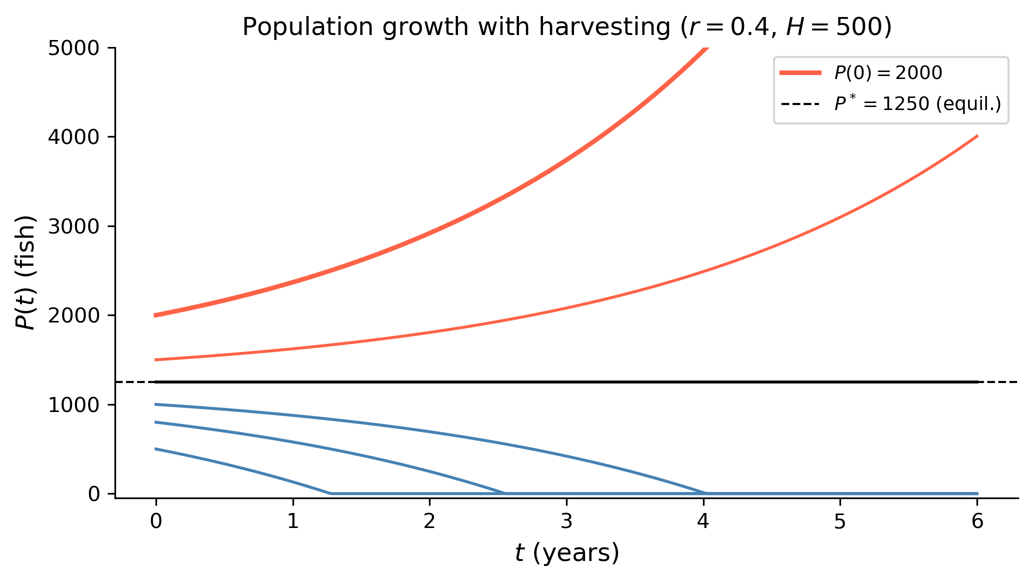
Long-term behavior. Since $e^{0.4t} \to \infty$, we have $P(t) \to \infty$; the population grows without bound because the growth rate $rP$ eventually outpaces the constant harvesting.

Tip

Equilibrium analysis. Setting $dP/dt = 0$ gives the equilibrium $P^* = H/r = 500/0.4 = 1250$ fish. Since the ODE $P' = 0.4(P - 1250)$ has an unstable equilibrium at $P^* = 1250$, populations starting above $1250$ (like our $P(0) = 2000$) grow without bound, while populations starting below $1250$ collapse to zero. Try the initial condition $P(0) = 1000$ to see the collapse!

Using SymPy

t  = sym.Symbol('t', nonnegative=True)
P  = sym.Function('P')
r, H_val = sym.Rational(2, 5), sym.Integer(500)  # r = 0.4, H = 500

ode5 = sym.Eq(P(t).diff(t), r * P(t) - H_val)

sol5 = sym.dsolve(ode5, P(t), ics={P(0): 2000})
display(Math(r'P(t) = ' + sym.latex(sol5.rhs)))

$\displaystyle P(t) = 750 e^{\frac{2 t}{5}} + 1250$

Show the code

t_plot = np.linspace(0, 6, 300)

fig, ax = plt.subplots(figsize=(7, 4))

for P0, color, lw, zord in [(500, 'steelblue', 1.4, 2),
                              (800, 'steelblue', 1.4, 2),
                              (1000,'steelblue', 1.4, 2),
                              (1250,'black',     1.4, 3),
                              (1500,'tomato',    1.4, 2),
                              (2000,'tomato',    2.2, 4)]:
    C_num = P0 - 1250
    P_sol = 1250 + C_num * np.exp(0.4 * t_plot)
    # Clip at 0 for display
    P_disp = np.maximum(P_sol, 0)
    label = f'$P(0)={P0}$' if P0 == 2000 else None
    ax.plot(t_plot, P_disp, color=color, lw=lw, zorder=zord, label=label)

ax.axhline(1250, color='black', ls='--', lw=1, label=r'$P^* = 1250$ (equil.)')
ax.set_xlabel(r'$t$ (years)', fontsize=12)
ax.set_ylabel(r'$P(t)$ (fish)', fontsize=12)
ax.set_title('Population growth with harvesting ($r=0.4$, $H=500$)', fontsize=12)
ax.set_ylim(-50, 5000)
ax.legend(fontsize=9)
plt.tight_layout()
plt.show()

Figure 4: Fish population under constant harvesting. Starting above the unstable equilibrium $P^* = 1250$, the population grows; starting below, it collapses. The red curve uses the given initial condition $P(0) = 2000$.

Example 6 — Application: Series RL Electric Circuit

A series RL circuit consists of a resistor $R = 4\ \Omega$, an inductor $L = 0.1$ H, and a voltage source $E(t) = 12\sin(10t)$ V. The initial current is $I(0) = 0$ A. Find the current $I(t)$ in the circuit.

By Hand

Kirchhoff’s Voltage Law applied to a series RL circuit gives \[ L\,\frac{dI}{dt} + RI = E(t), \] which we rewrite in standard linear form by dividing through by $L$: \[ \frac{dI}{dt} + \frac{R}{L}\,I = \frac{E(t)}{L}. \]

With the given values $R = 4$, $L = 0.1$, $E(t) = 12\sin(10t)$: \[ \frac{dI}{dt} + 40\,I = 120\sin(10t), \qquad I(0) = 0. \]

Step 1 — Compute the integrating factor.

\[ \mu(t) = e^{\int 40\,dt} = e^{40t}. \]

Step 2 — Multiply and integrate.

\[ \frac{d}{dt}\!\left[e^{40t} I\right] = 120\,e^{40t}\sin(10t). \]

We need $\displaystyle\int e^{40t}\sin(10t)\,dt$. Use the formula \[ \int e^{at}\sin(bt)\,dt = \frac{e^{at}}{a^2+b^2}\bigl(a\sin(bt) - b\cos(bt)\bigr) + C, \] with $a = 40$ and $b = 10$: \[ \int e^{40t}\sin(10t)\,dt = \frac{e^{40t}}{1600+100}\bigl(40\sin(10t) - 10\cos(10t)\bigr) + C = \frac{e^{40t}}{1700}\bigl(40\sin(10t) - 10\cos(10t)\bigr) + C. \]

Therefore \[ e^{40t} I = 120 \cdot \frac{e^{40t}}{1700}\bigl(40\sin(10t) - 10\cos(10t)\bigr) + C = \frac{120}{1700}\,e^{40t}\bigl(40\sin(10t) - 10\cos(10t)\bigr) + C. \]

Step 3 — Solve for $I(t)$.

Dividing by $e^{40t}$: \[ I(t) = \frac{120}{1700}\bigl(40\sin(10t) - 10\cos(10t)\bigr) + Ce^{-40t}. \]

Simplify $\dfrac{120}{1700} = \dfrac{12}{170} = \dfrac{6}{85}$: \[ I(t) = \frac{6}{85}\bigl(40\sin(10t) - 10\cos(10t)\bigr) + Ce^{-40t} = \frac{240}{85}\sin(10t) - \frac{60}{85}\cos(10t) + Ce^{-40t}. \]

Step 4 — Apply the initial condition $I(0) = 0$.

\[ 0 = \frac{240}{85}(0) - \frac{60}{85}(1) + C = -\frac{60}{85} + C \quad\Longrightarrow\quad C = \frac{60}{85} = \frac{12}{17}. \]

The particular solution is \[ \boxed{I(t) = \frac{240}{85}\sin(10t) - \frac{60}{85}\cos(10t) + \frac{12}{17}\,e^{-40t}.} \]

Steady-state and transient interpretation.

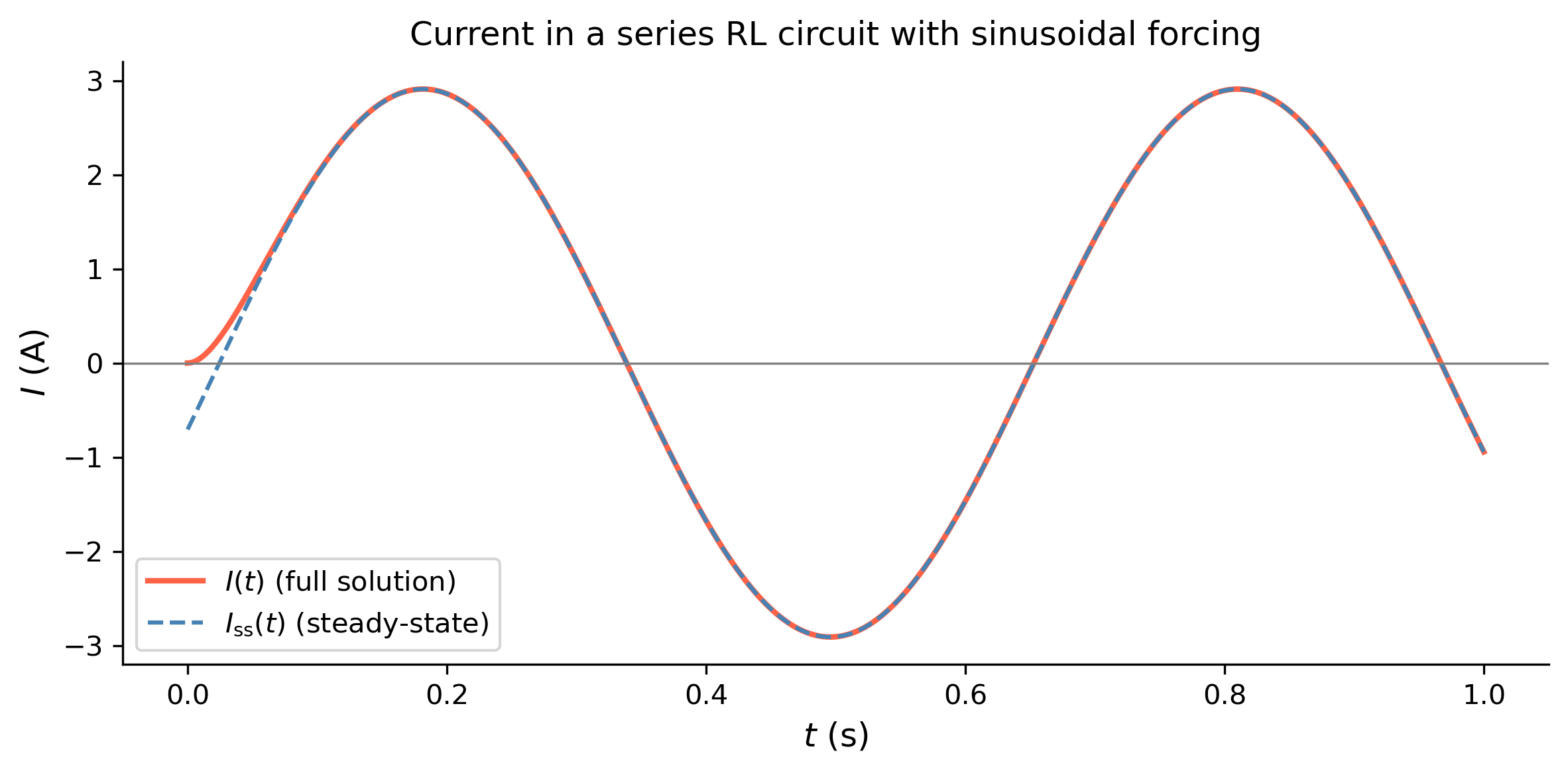
The term $\dfrac{12}{17}\,e^{-40t}$ is the transient part: it decays rapidly to zero (time constant $\tau = 1/40 = 0.025$ s). The remaining terms \[ I_{\text{ss}}(t) = \frac{240}{85}\sin(10t) - \frac{60}{85}\cos(10t) \] constitute the steady-state (forced) response, which oscillates at the driving frequency $\omega = 10$ rad/s. We can write this in amplitude–phase form:

\[ I_{\text{ss}}(t) = A\sin(10t + \phi), \]

where \[ A = \sqrt{\left(\frac{240}{85}\right)^2 + \left(\frac{60}{85}\right)^2} = \frac{1}{85}\sqrt{240^2 + 60^2} = \frac{60\sqrt{17}}{85} = \frac{12\sqrt{17}}{17} \approx 2.91\text{ A}. \]

Note

The time constant $\tau = L/R = 0.1/4 = 0.025$ s means the transient dies out within a fraction of a second — much faster than the period of the driving signal $T = 2\pi/10 \approx 0.63$ s.

Using SymPy

t = sym.Symbol('t', nonnegative=True)
I = sym.Function('I')
R_val, L_val = sym.Integer(4), sym.Rational(1, 10)

ode6 = sym.Eq(L_val * I(t).diff(t) + R_val * I(t),
              12 * sym.sin(10 * t))

sol6 = sym.dsolve(ode6, I(t), ics={I(0): 0})
I_expr = sym.simplify(sol6.rhs)
display(Math(r'I(t) = ' + sym.latex(I_expr)))

$\displaystyle I(t) = \frac{48 \sin{\left(10 t \right)}}{17} - \frac{12 \cos{\left(10 t \right)}}{17} + \frac{12 e^{- 40 t}}{17}$

Show the code

I_func = sym.lambdify(t, I_expr, 'numpy')
t_plot = np.linspace(0, 1.0, 1000)
I_plot = I_func(t_plot)

# Steady-state only
I_ss = (240/85) * np.sin(10 * t_plot) - (60/85) * np.cos(10 * t_plot)

fig, ax = plt.subplots(figsize=(8, 4))
ax.plot(t_plot, I_plot, color='tomato', lw=2,   label=r'$I(t)$ (full solution)')
ax.plot(t_plot, I_ss,  color='steelblue', lw=1.5, ls='--',
        label=r'$I_{\mathrm{ss}}(t)$ (steady-state)')
ax.axhline(0, color='gray', lw=0.8)
ax.set_xlabel(r'$t$ (s)', fontsize=12)
ax.set_ylabel(r'$I$ (A)', fontsize=12)
ax.set_title('Current in a series RL circuit with sinusoidal forcing', fontsize=12)
ax.legend(fontsize=10)
plt.tight_layout()
plt.show()

Figure 5: Current in the RL circuit. The transient decays quickly, leaving the sinusoidal steady-state response.

Expand for Session Info

import sys
print("Python version:", sys.version)
print('\n'.join(f'{m.__name__}=={m.__version__}'
                for m in globals().values()
                if getattr(m, '__version__', None)))

Python version: 3.14.4 | packaged by conda-forge | (main, Apr  8 2026, 02:33:53) [Clang 20.1.8 ]
numpy==2.4.3
sympy==1.14.0
matplotlib==3.10.8

Reuse

CC BY-NC-SA 4.0

Reuse

CC BY-NC-SA 4.0

Isocline \(y = x + c\)	Slope of segments
\(y = x - 2\)	\(-2\)
\(y = x - 1\)	\(-1\)
\(y = x\)	\(0\) (horizontal segments)
\(y = x + 1\)	\(1\)
\(y = x + 2\)	\(2\)