Notes 2

First-Order Equations

Show the code
# This is a code cell that imports the necessary libraries for our session.
import numpy as np                        # NumPy for numerical computations
import scipy as sp                        # SciPy for scientific computing
import sympy as sym                       # SymPy for symbolic mathematics
import matplotlib as mpl                  # Matplotlib for plotting
import matplotlib.pyplot as plt           # Matplotlib pyplot interface
from scipy.integrate import solve_ivp     # ODE solver
from IPython.display import Math, display
mpl.rcParams['figure.dpi'] = 150
mpl.rcParams['axes.spines.top'] = False
mpl.rcParams['axes.spines.right'] = False

Goals

In this section, we will cover the following topics:

  1. Define the notion of a first-order ODE and explain the slope-field concept as its geometric interpretation.

  2. Use slope fields, nullclines, and isoclines to sketch qualitative solution behavior without solving.

  3. Review the method of separation of variables for separable first-order equations.

  4. Study the class of first-order linear ODEs and introduce the method of integrating factors.

  5. Examine applications: Newton’s law of cooling (heat transfer) and RC circuits.

Note

This material corresponds to Sections 1.1.3, 1.3, and 1.4 of Logan (2015).

Slope Fields

The Geometric Idea

A first-order ODE of the form \[ x' = f(t, x) \] has a natural geometric interpretation. At any point \((t, x)\) in the plane, the ODE tells us the slope \(x'(t) = f(t, x(t))\) that a solution curve passing through that point must have. If we draw a short line segment at each point with the prescribed slope, the collection of all such segments is called the slope field (or direction field) of the equation.

Important

A slope field is a visualization of the ODE itself — before any solution has been found. Solution curves are precisely those curves that are everywhere tangent to the slope-field segments through which they pass.

In calculus, we are given a function and asked to find its derivative (slopes). Differential equations reverse this: we are given the slopes and asked to recover the function.


Nullclines and Isoclines

Two families of curves are especially useful for reading a slope field:

Nullclines. The set of points \((t, x)\) where \(f(t, x) = 0\), i.e., where the slope field is horizontal. Along a nullcline the solution curves have zero slope; in crossing a nullcline, solutions may change from increasing to decreasing (or vice versa). For an autonomous ODE \(x' = f(x)\), the nullclines are horizontal lines \(x = c\) where \(f(c) = 0\), and these are precisely the equilibrium (constant) solutions.

Isoclines. The set of points \((t, x)\) where \(f(t, x) = k\) for a fixed constant \(k\). Along an isocline all solution curves have the same slope \(k\). Plotting several isoclines gives a rapid sketch of how the slope field is organized.


Python: Drawing Slope Fields

Python’s matplotlib.pyplot.quiver function makes it straightforward to draw slope fields. The idea is to create a grid of \((t, x)\) points, evaluate \(f(t, x)\) at each point, and draw a unit-length arrow in the direction \((1, f(t,x))\) (normalized so all arrows have equal length).

A reusable helper function:

Show the code
def slope_field(f, t_range, x_range, n=20, ax=None, color='steelblue', alpha=0.7):
    """
    Draw the slope field for x' = f(t, x).

    Parameters
    ----------
    f        : callable  f(t, x) — the right-hand side of the ODE
    t_range  : (t_min, t_max)
    x_range  : (x_min, x_max)
    n        : grid resolution (n x n arrows)
    ax       : matplotlib Axes (creates one if None)
    color    : arrow color
    alpha    : arrow transparency
    """
    if ax is None:
        fig, ax = plt.subplots()
    t_vals = np.linspace(*t_range, n)
    x_vals = np.linspace(*x_range, n)
    T, X = np.meshgrid(t_vals, x_vals)
    dT = np.ones_like(T)          # dt component always 1
    dX = f(T, X)                  # dx component = f(t, x)
    # Normalize arrow lengths for visual clarity
    norm = np.sqrt(dT**2 + dX**2)
    norm[norm == 0] = 1
    ax.quiver(T, X, dT / norm, dX / norm,
              angles='xy', scale=n * 0.8, width=0.003,
              color=color, alpha=alpha, headlength=3, headwidth=3)
    ax.set_xlabel('$t$'); ax.set_ylabel('$x$')
    return ax

Example 1 — \(x' = -x + 2t\)

This is Example 1.5 in Logan (2015). The right-hand side is \(f(t, x) = -x + 2t\).

  • Nullcline: \(f = 0 \Rightarrow x = 2t\) (a line of slope 2).
  • Above the nullcline (\(x > 2t\)): \(f < 0\), slopes negative (solutions decreasing).
  • Below the nullcline (\(x < 2t\)): \(f > 0\), slopes positive (solutions increasing).
Show the code
f1 = lambda t, x: -x + 2*t

fig, ax = plt.subplots(figsize=(7, 5))
slope_field(f1, (-1, 4), (-4, 8), n=22, ax=ax)

# Several solution curves via solve_ivp
t_eval = np.linspace(-1, 4, 400)
for x0 in [-3, -1, 0, 2, 4, 6, 7.5]:
    sol = solve_ivp(f1, (-1, 4), [x0], t_eval=t_eval, max_step=0.05)
    ax.plot(sol.t, sol.y[0], color='steelblue', lw=1.8)

# Nullcline x = 2t
t_nc = np.linspace(-1, 4, 200)
ax.plot(t_nc, 2*t_nc, 'r--', lw=1.8, label='Nullcline $x = 2t$')

ax.set_xlim(-1, 4); ax.set_ylim(-4, 8)
ax.set_title(r"Slope field: $x' = -x + 2t$")
ax.legend()
plt.tight_layout()
plt.show()
Figure 1: Slope field for \(x' = -x + 2t\) with several solution curves (blue) and the nullcline \(x = 2t\) (red dashed). Solutions appear to converge toward the line \(x = 2t - 2\) — the particular solution that satisfies the ODE for all \(t\).

Example 2 — Autonomous ODE: \(x' = x(1 - x/4)\)

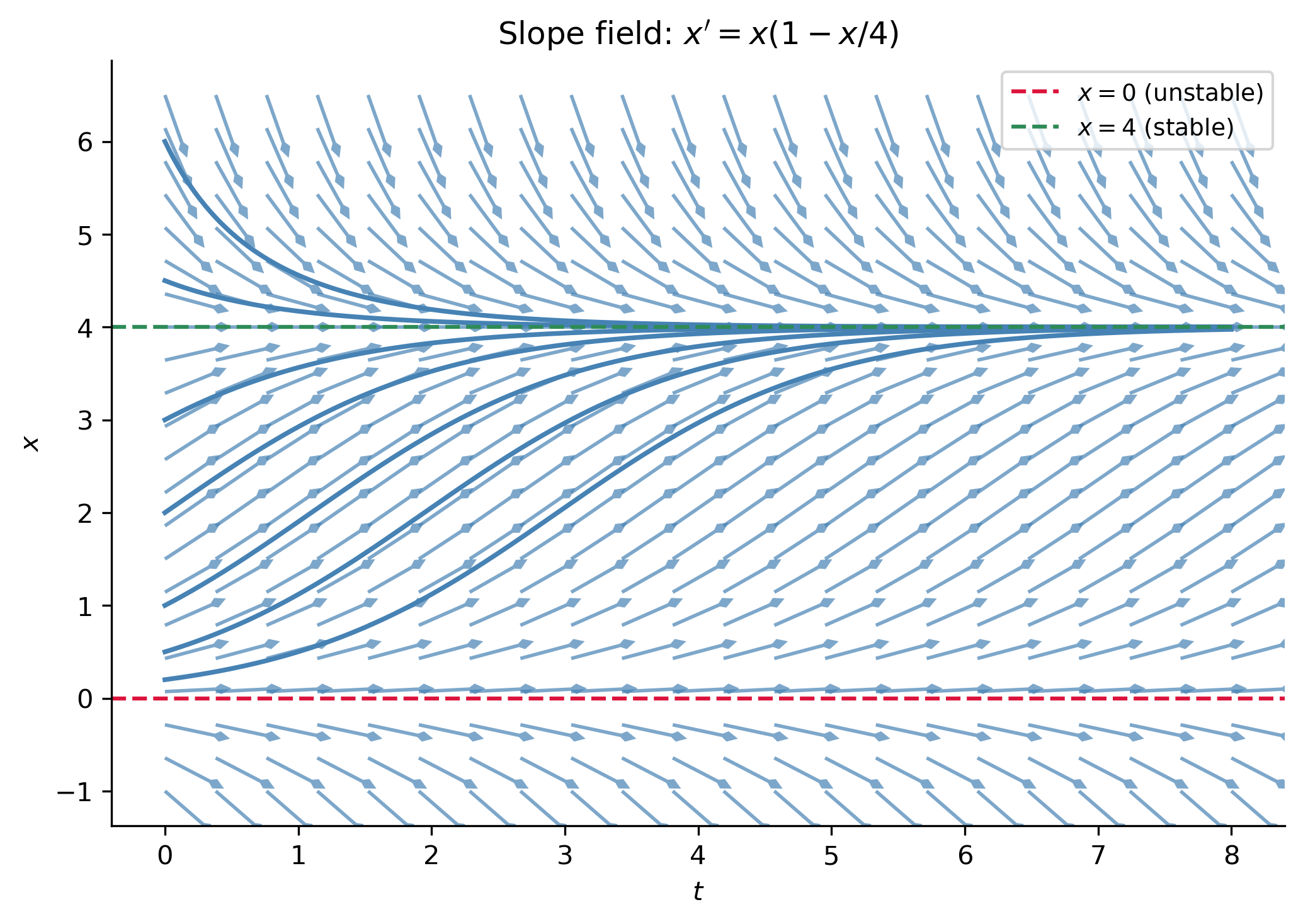
For an autonomous ODE \(x' = f(x)\), the slope field has a particularly simple structure: the slope is constant along each horizontal line \(x = c\). The nullclines are horizontal, and where \(f(c) = 0\) the line \(x = c\) is itself a constant (equilibrium) solution.

Here \(f(x) = x(1 - x/4)\). Setting \(f(x) = 0\) gives equilibria \(x = 0\) (unstable) and \(x = 4\) (stable).

Show the code
f2 = lambda t, x: x * (1 - x / 4)

fig, ax = plt.subplots(figsize=(7, 5))
slope_field(f2, (0, 8), (-1, 6.5), n=22, ax=ax)

t_eval = np.linspace(0, 8, 400)
for x0 in [0.2, 0.5, 1, 2, 3, 4.5, 6]:
    sol = solve_ivp(f2, (0, 8), [x0], t_eval=t_eval, max_step=0.05)
    ax.plot(sol.t, sol.y[0], color='steelblue', lw=1.8)

# Equilibria
ax.axhline(0, color='crimson', linestyle='--', lw=1.5, label='$x=0$ (unstable)')
ax.axhline(4, color='seagreen', linestyle='--', lw=1.5, label='$x=4$ (stable)')

ax.set_title(r"Slope field: $x' = x(1 - x/4)$")
ax.legend(fontsize=9)
plt.tight_layout()
plt.show()
Figure 2: Slope field for the autonomous ODE \(x' = x(1-x/4)\) (logistic-type). Horizontal dashed lines mark the nullclines/equilibria \(x=0\) and \(x=4\). All solutions starting with \(x_0 > 0\) converge to \(x=4\).
Tip

For any autonomous ODE \(x' = f(x)\), you can read off the qualitative behavior of all solutions directly from the sign of \(f(x)\): solutions increase where \(f(x) > 0\) and decrease where \(f(x) < 0\). This is the basis of the phase-line analysis we will develop in more detail later.


Example 3 — Nonlinear ODE: \(x' = x(x - t)\)

This is Example 1.6 in Logan (2015). The right-hand side is \(f(t, x) = x(x - t) = -tx + x^2\).

  • Nullclines: \(x = 0\) (the \(t\)-axis) and \(x = t\). Note that \(x(t) = 0\) is a constant solution; \(x = t\) is a nullcline but not a solution.
  • Four sign regions are separated by the two nullclines; see the plot annotations.
Show the code
f3 = lambda t, x: x * (x - t)

fig, ax = plt.subplots(figsize=(7, 5))
slope_field(f3, (-1, 4), (-3, 4.5), n=22, ax=ax)

t_eval = np.linspace(-1, 4, 600)
for x0, t0 in [(2.0, -1), (0.5, -1), (-1.5, -1), (3.5, -1)]:
    try:
        sol = solve_ivp(f3, (-1, 4), [x0], t_eval=t_eval, max_step=0.02,
                        events=lambda t, y: y[0] - 15)
        ax.plot(sol.t, np.clip(sol.y[0], -4, 5), color='steelblue', lw=1.8)
    except Exception:
        pass

t_nc = np.linspace(-1, 4, 200)
ax.axhline(0, color='crimson', linestyle='--', lw=1.8, label='Nullcline $x=0$')
ax.plot(t_nc, t_nc, color='darkorange', linestyle='--', lw=1.8, label='Nullcline $x=t$')

# Sign annotations
for txt, pos in [(r"$x'>0$", (2, -1.8)), (r"$x'<0$", (2, 0.6)),
                 (r"$x'>0$", (0.5, 2.5)), (r"$x'<0$", (-0.5, -1.5))]:
    ax.text(*pos, txt, fontsize=10, ha='center', color='black')

ax.set_xlim(-1, 4); ax.set_ylim(-3, 4.5)
ax.set_title(r"Slope field: $x' = x(x-t)$")
ax.legend(fontsize=9)
plt.tight_layout()
plt.show()
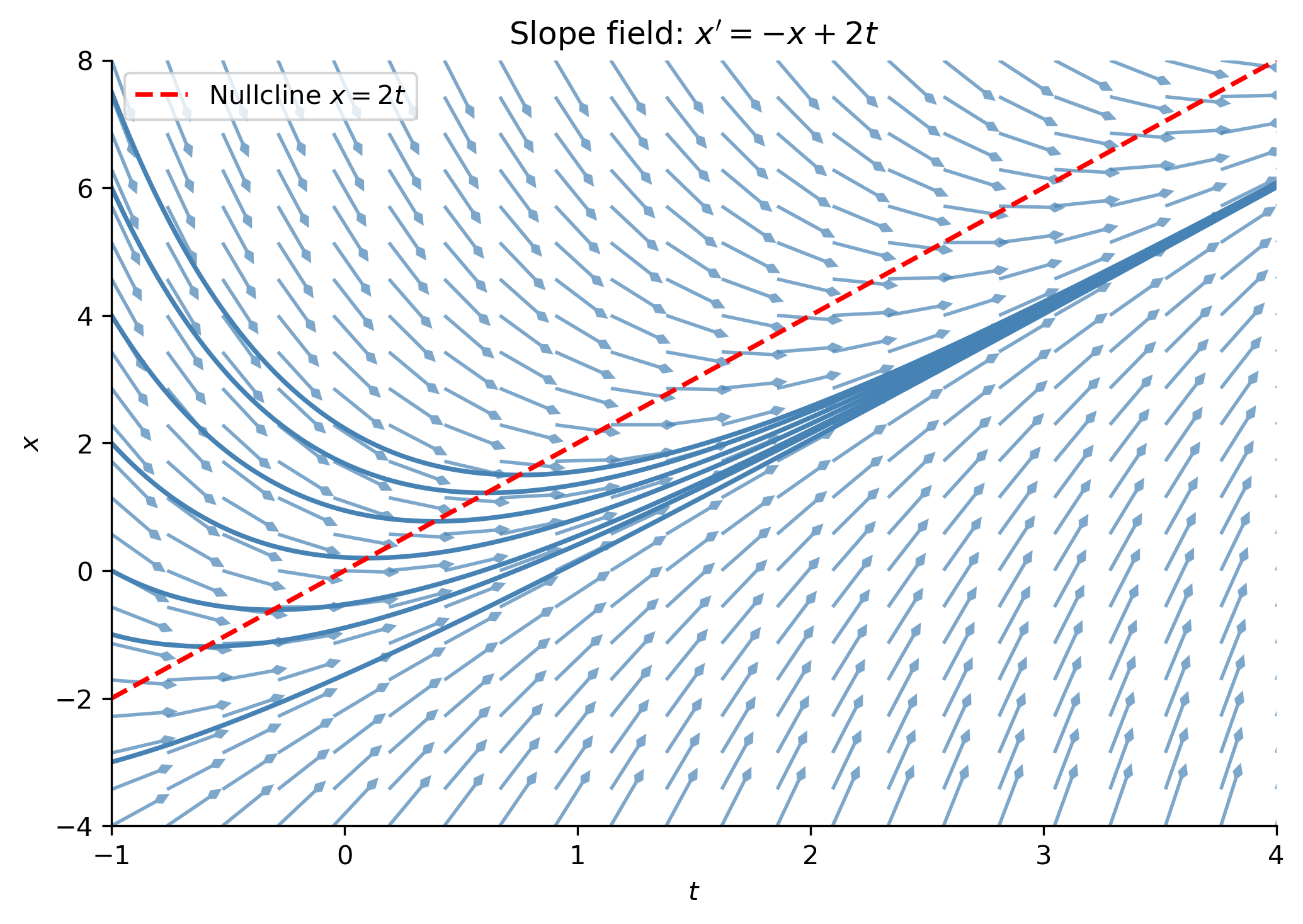
Figure 3: Slope field for \(x' = x(x-t)\) with nullclines \(x=0\) (red) and \(x=t\) (orange). Signs of \(x'\) in the four regions are annotated. Two approximate solution curves are shown in blue.

Separable Equations

Definition and Method

A first-order ODE is separable if it can be written in the form \[ x' = f(x)\,g(t), \] so that the right-hand side factors into a product of a function of \(x\) alone and a function of \(t\) alone.

The solution method — separation of variables — proceeds as follows. Writing \(x' = dx/dt\) and dividing by \(f(x)\): \[ \frac{1}{f(x)}\frac{dx}{dt} = g(t). \] Integrating both sides with respect to \(t\) and using the substitution \(dx = (dx/dt)\,dt\): \[ \boxed{\int \frac{1}{f(x)}\,dx = \int g(t)\,dt + C.} \] After computing the two integrals we obtain a one-parameter family of integral curves \(\phi(t, x) = C\) that define the solutions implicitly. If we can solve for \(x\) in terms of \(t\) we get an explicit solution; otherwise the solution is expressed implicitly.

Important

Recipe. For \(\dfrac{dx}{dt} = f(x)g(t)\), simply write \[ \frac{1}{f(x)}\,dx = g(t)\,dt \] and integrate both sides directly — there is no need to go through the intermediate step of integrating with respect to \(t\).

Tip

Definite-integral form. For an IVP with \(x(t_0) = x_0\) it is often cleaner to integrate with definite integrals: \[ \int_{x_0}^{x} \frac{1}{f(y)}\,dy = \int_{t_0}^{t} g(s)\,ds. \] No constant of integration is needed because the initial condition is already built in.


Example 4 — Exponential Growth/Decay

The equation \(\dfrac{dx}{dt} = rx\) (where \(r\) is a constant) is separable with \(f(x) = x\) and \(g(t) = r\). Separating: \[ \frac{1}{x}\,dx = r\,dt \quad\Longrightarrow\quad \ln|x| = rt + C \quad\Longrightarrow\quad x(t) = Ce^{rt}. \] This is the fundamental exponential growth/decay model. Applied to a population with \(x(0) = x_0\) it gives \(x(t) = x_0 e^{rt}\).

Let us verify this with SymPy.

Show the code
t, r, C, x0 = sym.symbols('t r C x_0', real=True, positive=True)
x = sym.Function('x')

ode = sym.Eq(x(t).diff(t), r * x(t))
sol = sym.dsolve(ode, x(t))
print("General solution:", sol)

sol_ivp = sym.dsolve(ode, x(t), ics={x(0): x0})
print("IVP solution (x(0)=x0):", sol_ivp)
General solution: Eq(x(t), C1*exp(r*t))
IVP solution (x(0)=x0): Eq(x(t), x_0*exp(r*t))

Example 5 — The Logistic Equation

\[ \frac{dx}{dt} = rx\!\left(1 - \frac{x}{K}\right), \qquad x(0) = x_0. \]

Separating variables and using partial fractions: \[ \frac{1}{x(K-x)}\,dx = \frac{r}{K}\,dt. \] Partial fractions: \(\dfrac{1}{x(K-x)} = \dfrac{1/K}{x} + \dfrac{1/K}{K-x}\). Integrating: \[ \frac{1}{K}\ln\left|\frac{x}{K-x}\right| = \frac{r}{K}\,t + C_1 \quad\Longrightarrow\quad \frac{x}{K-x} = Ce^{rt}. \] Solving for \(x\) and applying \(x(0) = x_0\): \[ \boxed{x(t) = \frac{K}{1 + \left(\dfrac{K}{x_0} - 1\right)e^{-rt}}.} \]

Show the code
t_s, r_s, K_s, x0_s = sym.symbols('t r K x_0', positive=True)
x_s = sym.Function('x')

logistic_ode = sym.Eq(x_s(t_s).diff(t_s), r_s * x_s(t_s) * (1 - x_s(t_s) / K_s))
sol_logistic = sym.dsolve(logistic_ode, x_s(t_s), ics={x_s(0): x0_s})
print("Logistic IVP solution:")
display(Math(sym.latex(sol_logistic)))
Logistic IVP solution:

\(\displaystyle x{\left(t \right)} = - \frac{K x_{0} e^{r t}}{\left(K - x_{0}\right) \left(- \frac{x_{0} e^{r t}}{K - x_{0}} - 1\right)}\)


Example 6 — A Separable Equation with a Non-Closed-Form Integral

Consider the IVP (Example 1.18 in Logan (2015)): \[ \frac{dx}{dt} = \frac{2\sqrt{x}\,e^{-t}}{t}, \qquad x(1) = 4. \] Separating: \(\dfrac{dx}{2\sqrt{x}} = \dfrac{e^{-t}}{t}\,dt\). Integrating from the initial condition: \[ \int_4^x \frac{dy}{2\sqrt{y}} = \int_1^t \frac{e^{-s}}{s}\,ds \quad\Longrightarrow\quad \sqrt{x} - 2 = \int_1^t \frac{e^{-s}}{s}\,ds. \] The right-hand side cannot be expressed in terms of elementary functions. The solution is therefore written implicitly as \[ x(t) = \left(\int_1^t \frac{e^{-s}}{s}\,ds + 2\right)^{\!2}. \] Despite its complicated appearance, it is easy to plot numerically.

Show the code
from scipy.integrate import quad

def x_formula(t_val):
    integral, _ = quad(lambda s: np.exp(-s) / s, 1, t_val)
    return (integral + 2)**2

t_plot = np.linspace(1, 5, 300)
x_plot = np.array([x_formula(tv) for tv in t_plot])

# Cross-check with direct ODE solve
f_ode = lambda t, x: 2 * np.sqrt(max(x[0], 0)) * np.exp(-t) / t
sol_check = solve_ivp(f_ode, (1, 5), [4.0], t_eval=t_plot, max_step=0.02)

fig, ax = plt.subplots(figsize=(7, 4))
ax.plot(t_plot, x_plot, color='steelblue', lw=2.5, label='Integral formula')
ax.plot(sol_check.t[::15], sol_check.y[0][::15], 'ro', markersize=5, label='Numerical ODE solve')
ax.plot(1, 4, 'k*', markersize=10, label='IC $(1, 4)$')
ax.set_xlabel('$t$'); ax.set_ylabel('$x(t)$')
ax.set_title(r"$x' = 2\sqrt{x}\,e^{-t}/t$, $x(1)=4$")
ax.legend()
plt.tight_layout()
plt.show()
Figure 4: Solution to the IVP \(x' = 2\sqrt{x}\,e^{-t}/t\), \(x(1)=4\), expressed via a non-elementary integral. The solid blue curve shows the formula; the red dots confirm it by comparing with a direct numerical ODE solve.

Singular Solutions

Separating variables requires dividing by \(f(x)\), which is only valid when \(f(x) \neq 0\). Any value \(x = c\) with \(f(c) = 0\) yields a constant solution \(x(t) \equiv c\) that may not be obtainable from the general family by any choice of \(C\) — a singular solution.

NoteExample 7 — Singular Solution

The ODE \(x' = 6t(x-1)^{2/3}\) has the general solution \(x(t) = 1 + (t^2 + C)^3\). But \(x(t) \equiv 1\) also satisfies the ODE (check: \(x' = 0\) and \(6t(1-1)^{2/3} = 0\) ✓), and no choice of \(C\) in the general family gives \(x(t) = 1\). So \(x = 1\) is a singular solution.

Linear Equations

Normal Form and the Integrating Factor Method

A first-order linear ODE in normal form is \[ x' + p(t)\,x = q(t). \tag{1} \] The function \(q(t)\) is called the forcing term (or source term). If \(q \equiv 0\) the equation is homogeneous; otherwise it is inhomogeneous (nonhomogeneous).

The key algebraic trick is to multiply both sides of (1) by the integrating factor \[ \mu(t) = e^{\int p(t)\,dt} = e^{P(t)}, \qquad P(t) = \int p(t)\,dt. \] By the product rule and the chain rule, \[ \mu(t)\bigl(x' + p(t)x\bigr) = \bigl(\mu(t)\,x\bigr)', \] so equation (1) becomes \[ \bigl(\mu(t)\,x\bigr)' = \mu(t)\,q(t). \] Integrating both sides and dividing by \(\mu(t)\) gives the general solution: \[ \boxed{x(t) = e^{-P(t)}\int e^{P(t)}\,q(t)\,dt + Ce^{-P(t)}.} \]

ImportantFour-Step Procedure
  1. Write the ODE in normal form: \(x' + p(t)x = q(t)\).
  2. Compute \(\mu(t) = e^{\int p(t)\,dt}\).
  3. Multiply through: \(\bigl(\mu x\bigr)' = \mu\,q(t)\).
  4. Integrate both sides, divide by \(\mu\), apply the initial condition.

Structure Theorem

The general solution of the inhomogeneous linear equation decomposes as \[ x(t) = x_h(t) + x_p(t), \] where: - \(x_h(t) = Ce^{-P(t)}\) is the general solution of the homogeneous equation \(x' + p(t)x = 0\), and - \(x_p(t) = e^{-P(t)}\int q(t)\,e^{P(t)}\,dt\) is a particular solution of the inhomogeneous equation.

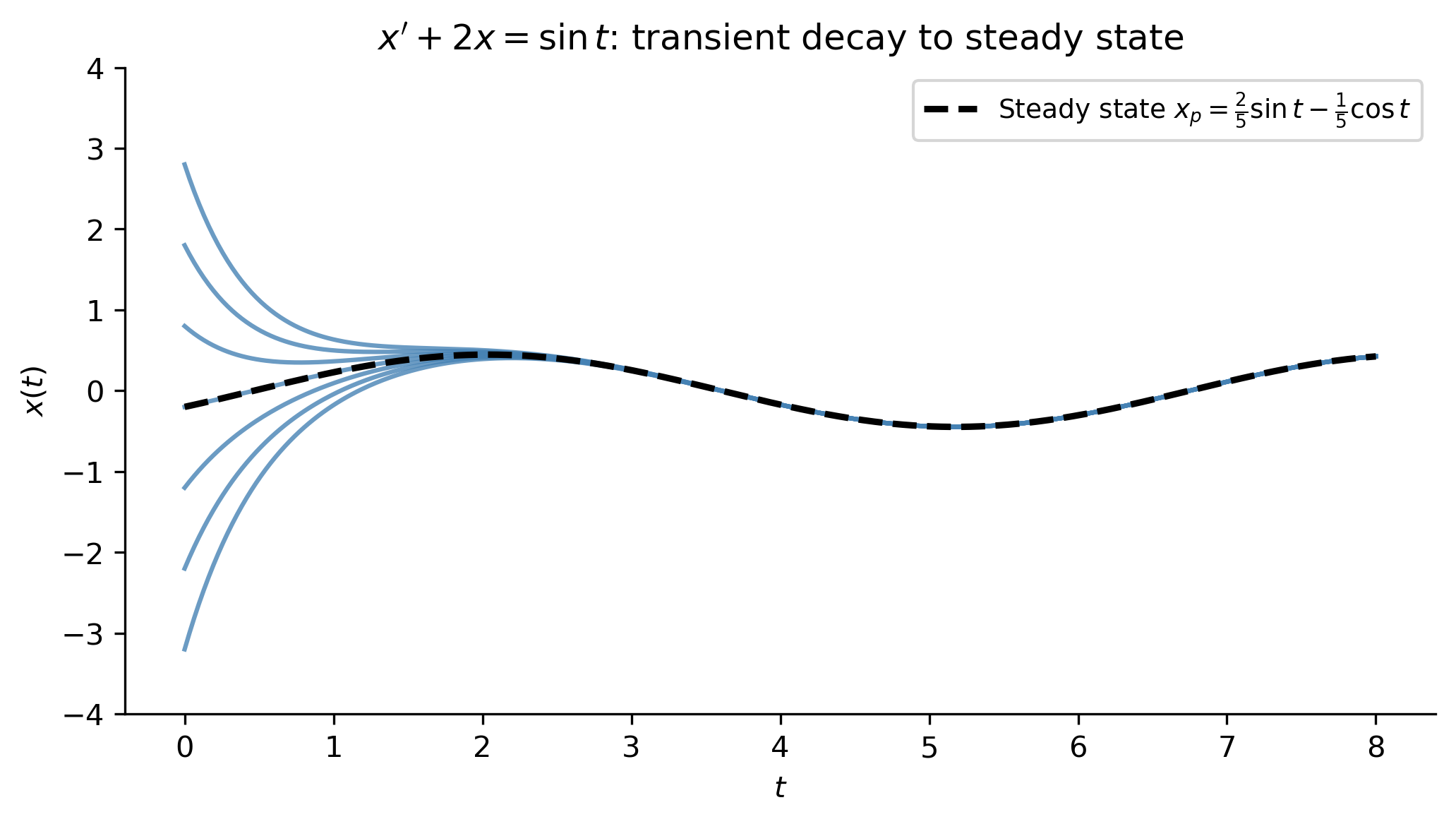
The homogeneous part \(x_h\) carries the initial condition (through \(C\)) and is often called the transient, because if \(P(t) \to \infty\) as \(t \to \infty\) it decays away. The particular part \(x_p\) is driven by \(q(t)\) and represents the steady-state response.


Example 8 — \(x' + \tfrac{1}{t}x = 1\)

Here \(p(t) = 1/t\) and \(q(t) = 1\).

Step 1. Already in normal form.

Step 2. \(\mu(t) = e^{\int (1/t)\,dt} = e^{\ln t} = t\).

Step 3. \((tx)' = t\).

Step 4. Integrate: \(tx = \tfrac{1}{2}t^2 + C\), so \[ x(t) = \frac{t}{2} + \frac{C}{t}. \]

If we impose \(x(1) = 3\): \(\tfrac{1}{2} + C = 3 \Rightarrow C = \tfrac{5}{2}\), giving \(x(t) = \tfrac{t}{2} + \tfrac{5}{2t}\).

Show the code
t_plot = np.linspace(0.2, 5, 400)
fig, ax = plt.subplots(figsize=(7, 4))
for C_val in np.linspace(-6, 6, 13):
    ax.plot(t_plot, t_plot/2 + C_val/t_plot, color='lightsteelblue', lw=0.9, alpha=0.8)
# Particular solution C = 5/2
ax.plot(t_plot, t_plot/2 + 2.5/t_plot, color='steelblue', lw=2.5, label=r'$C=5/2$, $x(1)=3$')
ax.plot(1, 3, 'ro', markersize=8, zorder=5, label='IC $(1, 3)$')
ax.set_ylim(-4, 8); ax.set_xlabel('$t$'); ax.set_ylabel('$x(t)$')
ax.set_title(r"$x' + x/t = 1$: general solution family")
ax.legend()
plt.tight_layout()
plt.show()
Figure 5: General solution \(x(t) = t/2 + C/t\) of \(x' + x/t = 1\) for several values of \(C\) (gray), with the particular solution satisfying \(x(1)=3\) highlighted (blue). The initial condition is marked in red.

Example 9 — \(x' + 2x = \sin t\)

Here \(p(t) = 2\) and \(q(t) = \sin t\).

Integrating factor: \(\mu(t) = e^{2t}\).

Multiply through: \((xe^{2t})' = e^{2t}\sin t\).

Integrate using integration by parts (or a table): \[ \int e^{2t}\sin t\,dt = e^{2t}\!\left(\tfrac{2}{5}\sin t - \tfrac{1}{5}\cos t\right) + \text{const}. \] Therefore the general solution is \[ x(t) = \frac{2}{5}\sin t - \frac{1}{5}\cos t + Ce^{-2t}. \]

Let us verify and plot this with SymPy.

Show the code
t_s = sym.Symbol('t')
x_s = sym.Function('x')
ode2 = sym.Eq(x_s(t_s).diff(t_s) + 2*x_s(t_s), sym.sin(t_s))
gen_sol = sym.dsolve(ode2, x_s(t_s))
print("General solution:")
display(Math(sym.latex(gen_sol)))

# Numerical plot
t_plot = np.linspace(0, 8, 500)
xp = 0.4*np.sin(t_plot) - 0.2*np.cos(t_plot)   # particular solution

fig, ax = plt.subplots(figsize=(7, 4))
for C_val in [-3, -2, -1, 0, 1, 2, 3]:
    x_sol = xp + C_val * np.exp(-2 * t_plot)
    ax.plot(t_plot, x_sol, color='steelblue', lw=1.5, alpha=0.8)
ax.plot(t_plot, xp, 'k--', lw=2.2, label=r'Steady state $x_p = \frac{2}{5}\sin t - \frac{1}{5}\cos t$')
ax.set_xlabel('$t$'); ax.set_ylabel('$x(t)$'); ax.set_ylim(-4, 4)
ax.set_title(r"$x' + 2x = \sin t$: transient decay to steady state")
ax.legend(fontsize=9)
plt.tight_layout()
plt.show()
General solution:

\(\displaystyle x{\left(t \right)} = C_{1} e^{- 2 t} + \frac{2 \sin{\left(t \right)}}{5} - \frac{\cos{\left(t \right)}}{5}\)

(a) Solutions of \(x' + 2x = \sin t\) for various initial conditions. The transient \(Ce^{-2t}\) decays quickly and all solutions converge to the same steady-state oscillation \(x_p = \frac{2}{5}\sin t - \frac{1}{5}\cos t\) (dashed black).
(b)
Figure 6

Applications

Newton’s Law of Cooling

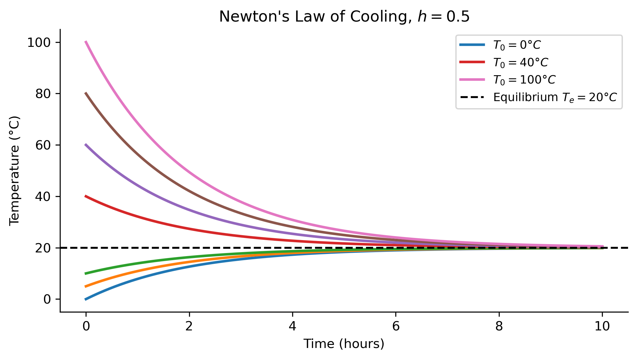
Newton’s law of cooling states that the rate of change of temperature of an object is proportional to the difference between the object’s temperature \(T\) and the ambient (environmental) temperature \(T_e\): \[ \frac{dT}{dt} = -h(T - T_e), \qquad T(0) = T_0, \] where \(h > 0\) is the heat loss coefficient. This is a first-order linear ODE (it is also separable). Writing it in normal form: \[ T' + hT = hT_e. \] The integrating factor is \(\mu = e^{ht}\), giving \((Te^{ht})' = hT_e e^{ht}\), and integrating: \[ T(t) = T_e + (T_0 - T_e)\,e^{-ht}. \] As \(t \to \infty\), \(T(t) \to T_e\) regardless of \(T_0\) — the object reaches thermal equilibrium with its environment. The equilibrium \(T = T_e\) is stable.

Variable ambient temperature. If \(T_e\) is replaced by a time-dependent function \(Q(t)\) the ODE becomes \[ T' + hT = hQ(t), \] whose general solution is \[ T(t) = Ce^{-ht} + e^{-ht}\int_0^t hQ(s)\,e^{hs}\,ds. \]

Show the code
h_val = 0.5
Te = 20.0
t_plot = np.linspace(0, 10, 300)

fig, ax = plt.subplots(figsize=(7, 4))
for T0 in [0, 5, 10, 40, 60, 80, 100]:
    T_sol = Te + (T0 - Te) * np.exp(-h_val * t_plot)
    ax.plot(t_plot, T_sol, lw=2,
            label=f'$T_0 = {T0}°C$' if T0 in [0, 40, 100] else None)
ax.axhline(Te, color='black', linestyle='--', lw=1.5,
           label=f'Equilibrium $T_e = {int(Te)}°C$')
ax.set_xlabel('Time (hours)'); ax.set_ylabel('Temperature (°C)')
ax.set_title(r"Newton's Law of Cooling, $h=0.5$")
ax.legend(fontsize=9)
plt.tight_layout()
plt.show()
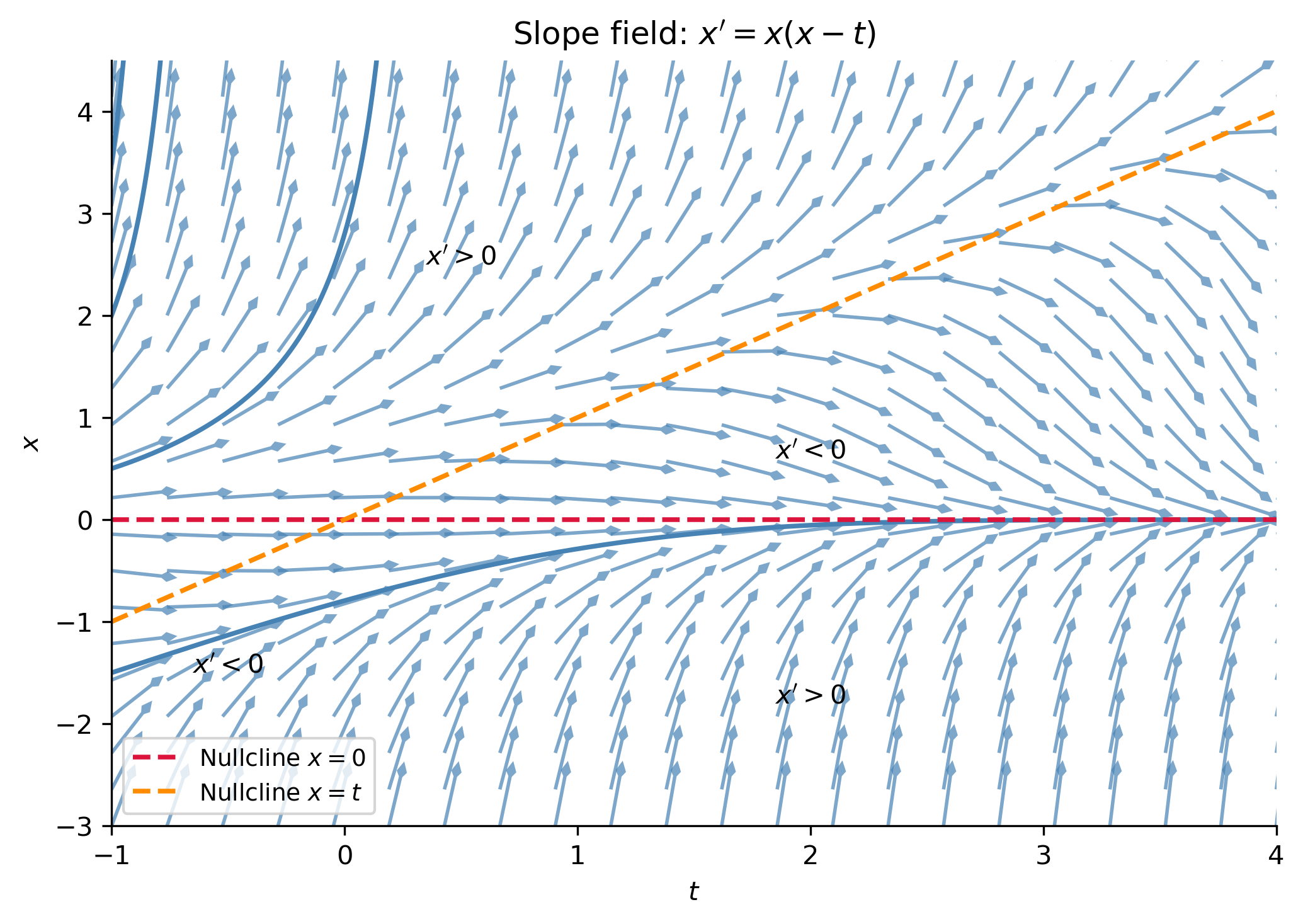
Figure 7: Newton’s law of cooling: temperature \(T(t) = T_e + (T_0 - T_e)e^{-ht}\) for \(T_e = 20^\circ\)C and \(h=0.5\) hr\(^{-1}\), starting from several initial temperatures. All curves converge to the equilibrium \(T_e = 20^\circ\)C (dashed).
NoteForensic Application

One classic application of Newton’s law of cooling is estimating the time of death from a body’s temperature. If a body at \(37°C\) is found in a \(20°C\) room at temperature \(T_1\) at time \(t_1\), and later at temperature \(T_2\) at time \(t_2\), then \(h\) can be estimated from the two measurements, and the time of death recovered by solving \(T(t_{\text{death}}) = 37°C\).


The RC Circuit

An RC circuit contains a resistor (\(R\)) and a capacitor (\(C\)) in series with a voltage source \(E(t)\). Kirchhoff’s voltage law and Ohm’s law give the first-order linear ODE for the charge \(Q(t)\) on the capacitor: \[ R\,Q' + \frac{Q}{C} = E(t) \quad\Longrightarrow\quad Q' + \frac{1}{RC}\,Q = \frac{E(t)}{R}. \] The integrating factor is \(\mu = e^{t/(RC)}\), giving the general solution \[ Q(t) = e^{-t/(RC)}\int_0^t \frac{E(s)}{R}\,e^{s/(RC)}\,ds + Q_0\,e^{-t/(RC)}, \] where \(Q_0 = Q(0)\).

Current. Since \(I = Q'\), differentiating gives the current \(I(t)\) once \(Q(t)\) is known.

The time constant \(\tau = RC\) governs how quickly the circuit charges/discharges:

  • Small \(\tau\): fast response.
  • Large \(\tau\): slow response.

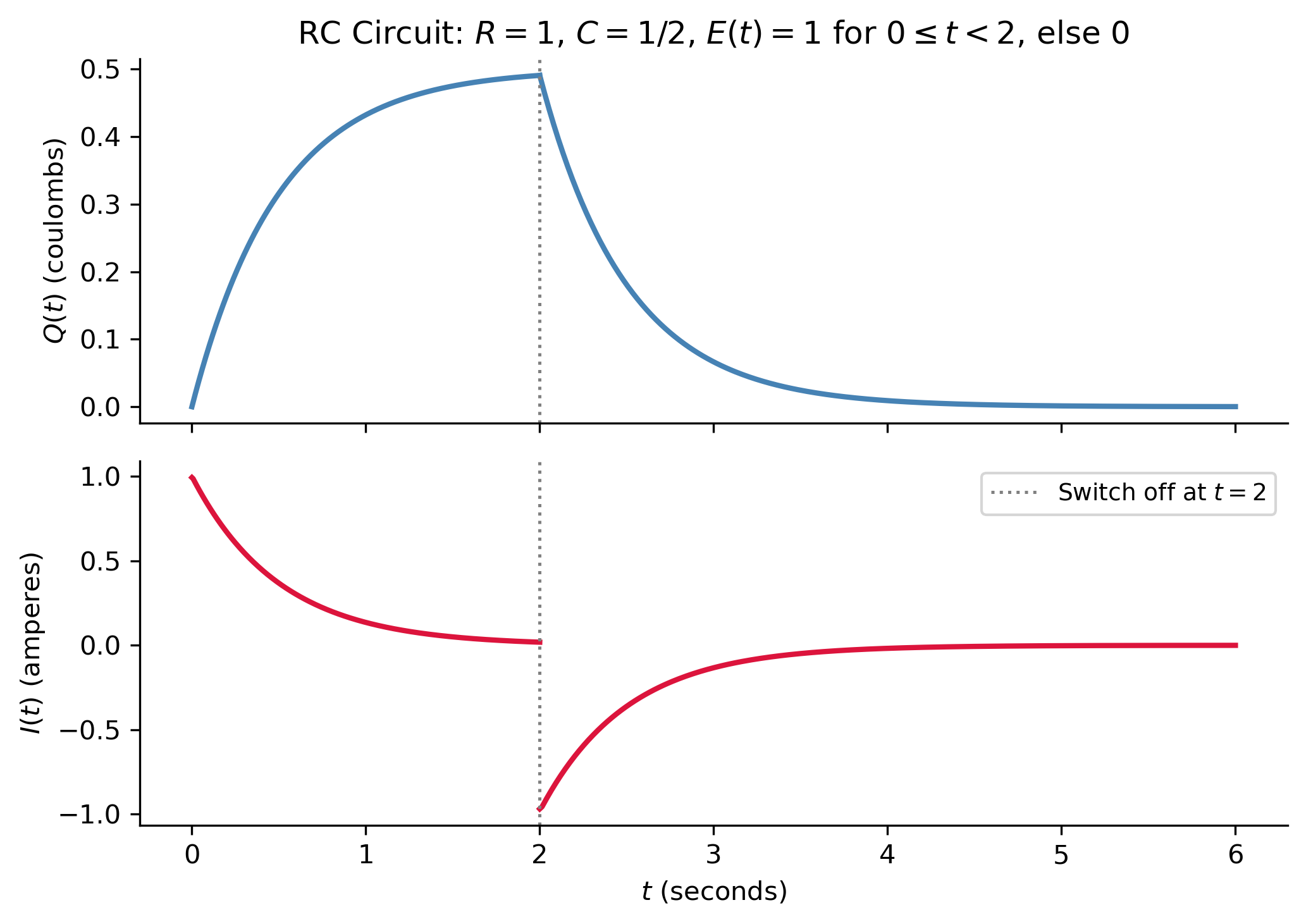
Piecewise forcing: switching on then off. The following example, based on Example 1.29 of Logan (2015), shows a circuit with \(R=1\), \(C=1/2\) (so \(\tau = 1/2\)), \(Q(0)=0\), and \[ E(t) = \begin{cases} 1, & 0 \leq t < 2 \\ 0, & t \geq 2. \end{cases} \]

For \(t < 2\): \(Q' + 2Q = 1\) with \(Q(0)=0\) gives \(Q_1(t) = \tfrac{1}{2}(1 - e^{-2t})\).

For \(t \geq 2\): \(Q' + 2Q = 0\) with \(Q(2) = Q_1(2)\) gives \(Q_2(t) = \tfrac{1}{2}(1 - e^{-4})\,e^{-2(t-2)}\).

Show the code
R_val, C_val = 1.0, 0.5
tau = R_val * C_val     # = 0.5
Q0 = 0.0

t1 = np.linspace(0, 2, 300)
t2 = np.linspace(2, 6, 300)

Q1 = 0.5 * (1 - np.exp(-2 * t1))
Q_switch = 0.5 * (1 - np.exp(-4))           # Q at t=2, matching condition
Q2 = Q_switch * np.exp(-2 * (t2 - 2))

I1 = np.gradient(Q1, t1)
I2 = np.gradient(Q2, t2)

fig, axes = plt.subplots(2, 1, figsize=(7, 5), sharex=True)

axes[0].plot(t1, Q1, color='steelblue', lw=2)
axes[0].plot(t2, Q2, color='steelblue', lw=2)
axes[0].axvline(2, color='gray', linestyle=':', lw=1.2)
axes[0].set_ylabel('$Q(t)$ (coulombs)')
axes[0].set_title(r'RC Circuit: $R=1$, $C=1/2$, $E(t)=1$ for $0\leq t<2$, else $0$')

axes[1].plot(t1, I1, color='crimson', lw=2)
axes[1].plot(t2, I2, color='crimson', lw=2)
axes[1].axvline(2, color='gray', linestyle=':', lw=1.2, label='Switch off at $t=2$')
axes[1].set_ylabel('$I(t)$ (amperes)')
axes[1].set_xlabel('$t$ (seconds)')
axes[1].legend(fontsize=9)

plt.tight_layout()
plt.show()
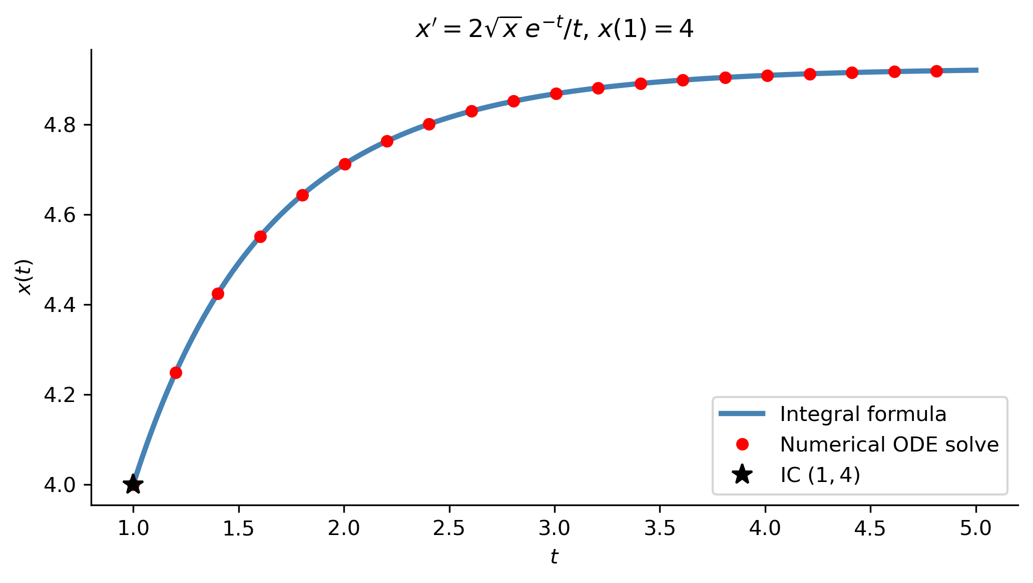
Figure 8: RC circuit (\(R=1\), \(C=1/2\)) with the voltage source switched on for \(0 \le t < 2\) then switched off. Top: charge \(Q(t)\). Bottom: current \(I(t) = Q'(t)\). Both confirm the matching condition at \(t=2\) and the characteristic exponential transient with time constant \(\tau = RC = 1/2\).
Tip

The mechanical–electrical analogy noted in Notes 1 now becomes concrete: the RC circuit equation \(Q' + Q/(RC) = E(t)/R\) is identical in form to Newton’s law of cooling \(T' + hT = hT_e(t)\) with the correspondence \(RC \leftrightarrow 1/h\) and \(E(t)/R \leftrightarrow hT_e(t)\). Solutions to both have the same transient + steady-state structure.


Chemical Mixture (Chemostat)

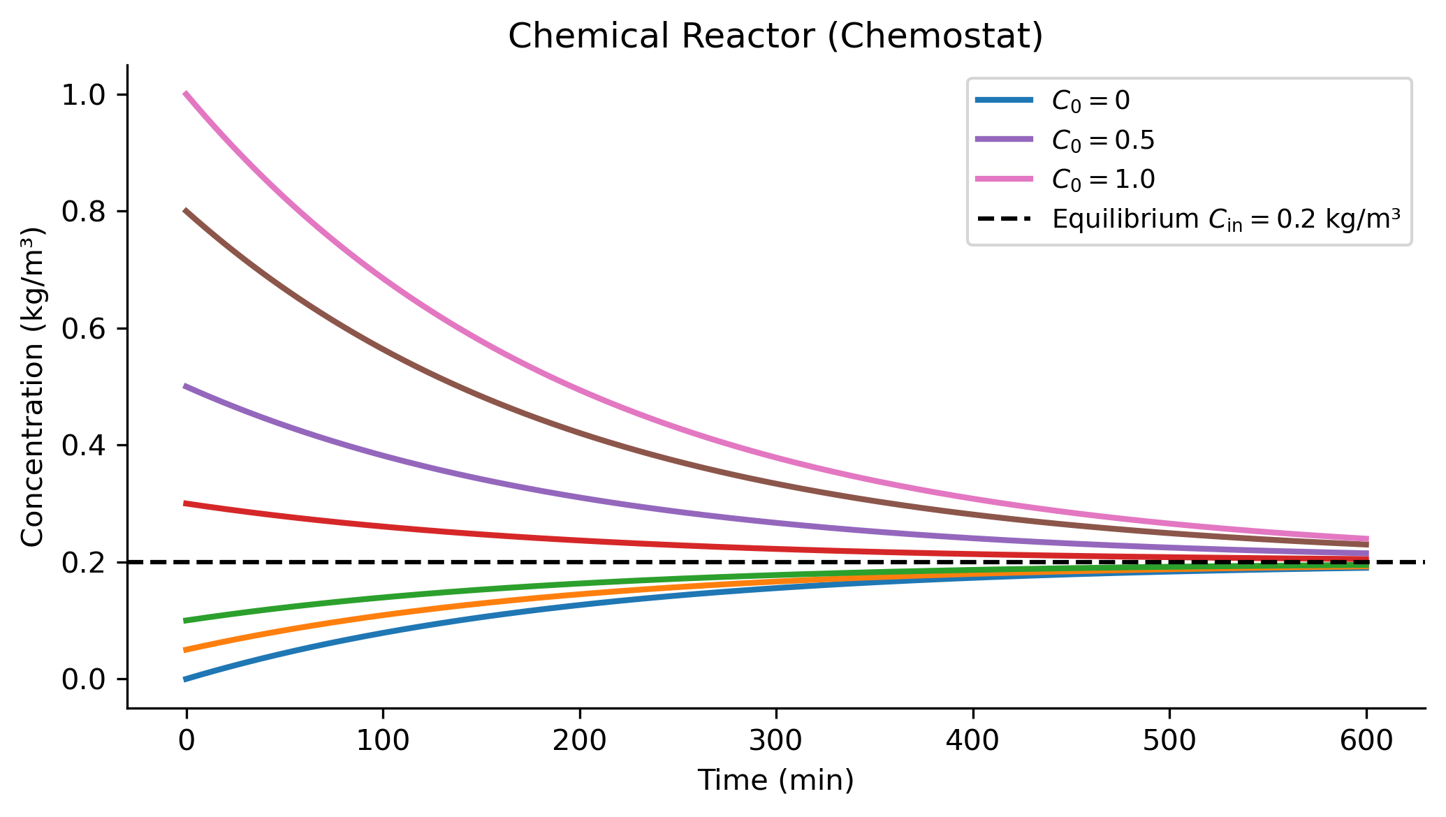
A well-mixed tank (reactor) of constant volume \(V\) has a chemical of concentration \(C(t)\). Contaminated inflow at concentration \(C_{\text{in}}\) enters at volumetric rate \(q\), and the well-mixed solution exits at the same rate. Mass balance (rate of change = rate in \(-\) rate out) gives: \[ V\,C' = q\,C_{\text{in}} - q\,C \quad\Longrightarrow\quad C' + \frac{q}{V}\,C = \frac{q}{V}\,C_{\text{in}}. \] This is a first-order linear ODE with \(p = q/V\) and \(q_{\text{forcing}} = (q/V)C_{\text{in}}\). The integrating factor is \(e^{qt/V}\), and with \(C(0) = C_0\) the solution is \[ C(t) = C_{\text{in}} + (C_0 - C_{\text{in}})\,e^{-qt/V}. \] As \(t \to \infty\), \(C(t) \to C_{\text{in}}\), the inflow concentration — the equilibrium is stable regardless of the initial concentration.

Show the code
V_val = 100.0     # m^3
q_vol = 0.5       # m^3/min
C_in  = 0.2       # kg/m^3
t_plot = np.linspace(0, 600, 500)

fig, ax = plt.subplots(figsize=(7, 4))
for C0 in [0, 0.05, 0.1, 0.3, 0.5, 0.8, 1.0]:
    C_sol = C_in + (C0 - C_in) * np.exp(-q_vol / V_val * t_plot)
    ax.plot(t_plot, C_sol, lw=2,
            label=f'$C_0={C0}$' if C0 in [0, 0.5, 1.0] else None)
ax.axhline(C_in, color='black', linestyle='--', lw=1.5,
           label=f'Equilibrium $C_{{\\rm in}}={C_in}$ kg/m³')
ax.set_xlabel('Time (min)'); ax.set_ylabel('Concentration (kg/m³)')
ax.set_title('Chemical Reactor (Chemostat)')
ax.legend(fontsize=9)
plt.tight_layout()
plt.show()
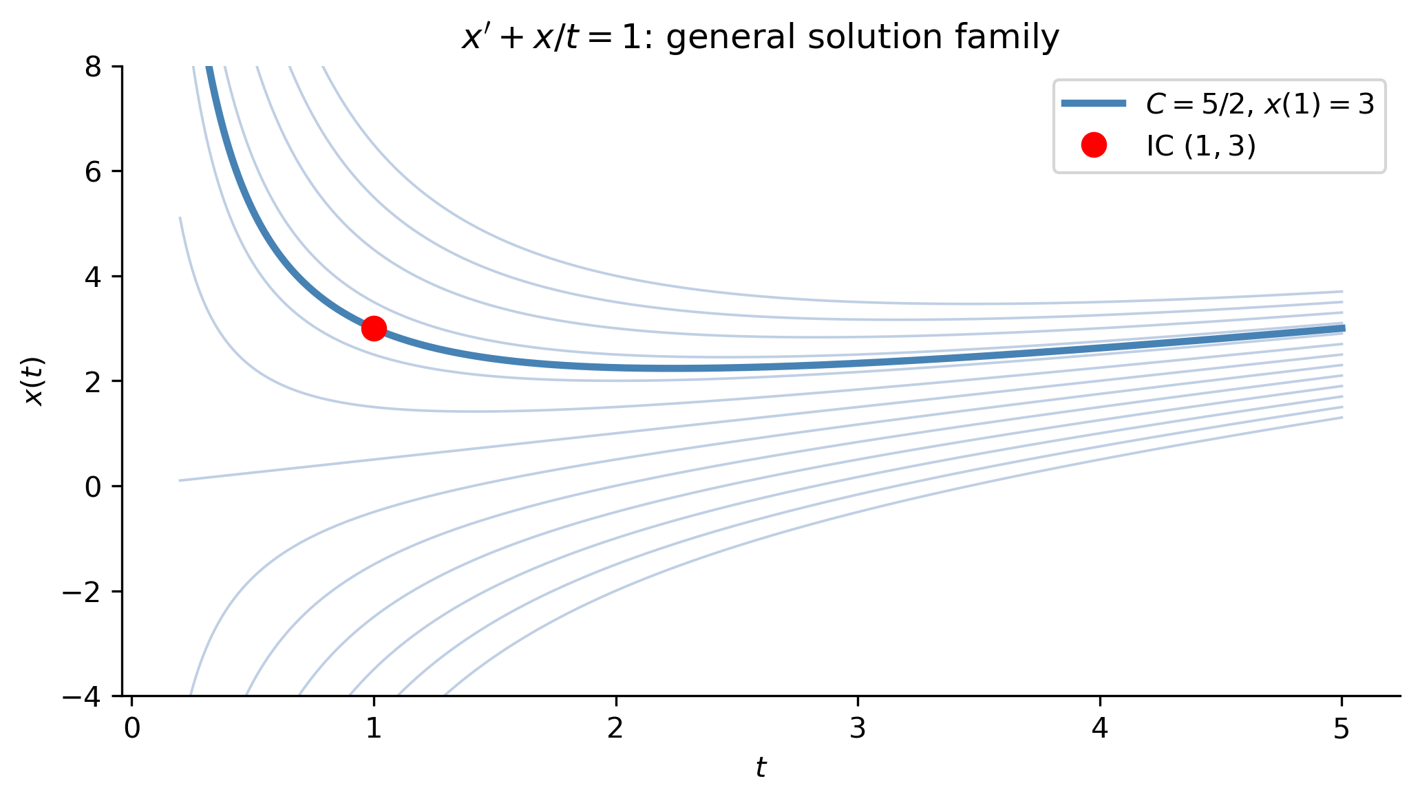
Figure 9: Chemical concentration in a well-mixed tank (\(V=100\) m\(^3\), \(q=0.5\) m\(^3\)/min, \(C_{\text{in}} = 0.2\) kg/m\(^3\)) for several initial concentrations \(C_0\). All solutions converge to the equilibrium \(C_{\text{in}} = 0.2\) (dashed).

Summary

Key Takeaways

  • A slope field visualizes \(x'=f(t,x)\) geometrically. Nullclines (\(f=0\)) and isoclines (\(f=k\)) organize the field and identify equilibria.

  • An ODE is separable if \(x' = f(x)g(t)\). Write \(\frac{dx}{f(x)} = g(t)\,dt\) and integrate. Watch for singular solutions at roots of \(f\).

  • A first-order linear ODE \(x'+p(t)x=q(t)\) is solved by the integrating factor \(\mu=e^{\int p\,dt}\). The solution always decomposes as transient (\(x_h\)) + steady state (\(x_p\)).

  • Newton’s cooling, RC circuits, and chemostats are all governed by the same first-order linear ODE — same structure, same solution formula, different physical interpretations.

These notes are also viewable as a slide deck presentation: Open slides in full screen

Note

Next: One-dimensional dynamical systems, equilibria and stability — Logan §1.5.


Relevant Videos

Slope fields:

Separation of variables:

Linear equations and integrating factor:

References

Logan, J David. 2015. A First Course in Differential Equations Third Edition.
Show the code
import sys # sys for system-specific parameters and functions
print("Python version:", sys.version)
print('\n'.join(f'{m.__name__}=={m.__version__}' for m in globals().values() if getattr(m, '__version__', None)))
Python version: 3.14.4 | packaged by conda-forge | (main, Apr  8 2026, 02:33:53) [Clang 20.1.8 ]
numpy==2.4.3
scipy==1.17.1
sympy==1.14.0
matplotlib==3.10.8