Notes 9

Linear Systems and Matrices

Show the code
import numpy as np
import sympy as sym
import matplotlib as mpl
import matplotlib.pyplot as plt
from scipy.integrate import solve_ivp
from IPython.display import Math, display
mpl.rcParams['figure.dpi'] = 150
mpl.rcParams['axes.spines.top'] = False
mpl.rcParams['axes.spines.right'] = False

Goals

  1. Understand how a second-order linear ODE is equivalent to a planar first-order system via the substitution \(y = x'\).

  2. Recognize the Hamiltonian formulation of classical mechanics and how it naturally produces a first-order system for any mechanical oscillator.

  3. Master the general technique of reducing an \(n\)-th order ODE to an \(n\)-dimensional first-order system (the companion system).

  4. Visualize solutions of planar systems via time-series (component) plots and phase-plane orbits, and understand the role of nullclines and the vector field.

  5. Understand the method of elimination — converting a system back to a single second-order ODE — and use it to find general solutions.

  6. State and use the Superposition, Uniqueness, and General Solution theorems for linear systems.

  7. Carry out \(2\times 2\) matrix arithmetic — addition, scalar multiplication, multiplication, inverse, determinant — in support of the matrix formulation \(\mathbf{x}' = A\mathbf{x}\).

  8. Find equilibria (critical points) of linear and nonhomogeneous linear systems and interpret their stability.

Note

This material corresponds to Sections 4.1 and 4.2 of (Logan 2015).


Part 1 — Section 4.1: Linear Systems vs. Second-Order Equations

From Second-Order ODE to First-Order System

The damped oscillator equation \[mx'' + \gamma x' + kx = 0\] involves the second derivative of a single unknown \(x = x(t)\). If we introduce the velocity \[y = y(t) = x'(t)\] as a second dependent variable, then \(x' = y\) and the equation becomes \(my' = -kx - \gamma y\), giving the equivalent planar first-order system: \[\begin{cases} x' = y, \\[4pt] y' = -\dfrac{k}{m}x - \dfrac{\gamma}{m}y. \end{cases} \tag{4.1--4.2}\] This is a system of two first-order equations in two unknowns \(x(t)\) and \(y(t)\).

ImportantRemark 4.1 (Logan)

We can always reduce a second-order linear equation \(ax'' + bx' + cx = 0\) to a first-order linear system by defining \(y = x'\). The resulting system is completely equivalent to the original equation.

The Hamiltonian Perspective

The substitution \(y = x'\) acquires deep physical meaning in the Hamiltonian formulation of classical mechanics. For a particle of mass \(m\) with position \(q\) and momentum \(p = m\dot{q}\), the Hamiltonian (total energy) is \[H(q,p) = \underbrace{\frac{p^2}{2m}}_{\text{kinetic}} + \underbrace{V(q)}_{\text{potential}}.\]

Hamilton’s equations of motion are: \[\boxed{\dot{q} = \frac{\partial H}{\partial p} = \frac{p}{m}, \qquad \dot{p} = -\frac{\partial H}{\partial q} = -V'(q).}\]

These are exactly two coupled first-order ODEs. For the simple harmonic oscillator with \(V(q) = \frac{1}{2}kq^2\): \[\dot{q} = \frac{p}{m}, \qquad \dot{p} = -kq.\]

Setting \(m=1\) and writing \((x,y) = (q,p)\) with \(k=4\): \[x' = y, \qquad y' = -4x.\] This is precisely Example 4.3 and 4.4 in Logan, and the Hamiltonian is a conserved quantity along every orbit: \[H = \frac{1}{2}p^2 + \frac{1}{2}kq^2 = \frac{y^2}{2} + 2x^2 = C.\] These level curves are ellipses — exactly the phase-plane orbits of the system.

TipWhy the Hamiltonian Formulation Matters

The Hamiltonian approach is not merely a notational convenience. It reveals: 1. Energy conservation as a geometric property — orbits are level curves of \(H\). 2. Symplectic structure — the system \(\dot{\mathbf{z}} = J\nabla H\) (where \(J=\bigl[\begin{smallmatrix}0&1\\-1&0\end{smallmatrix}\bigr]\)) preserves phase-space area. 3. Generalizability to coupled oscillators, field theories, and quantum mechanics.

For the damped oscillator with \(\gamma > 0\), \(H\) is no longer conserved: \(\dot{H} = -\gamma(x')^2 \leq 0\) (energy is dissipated), which corresponds to spiraling orbits converging to the origin.

Show the code
t_plot = np.linspace(0, 2*np.pi, 400)
x_sol  = np.cos(2*t_plot)
y_sol  = -2*np.sin(2*t_plot)

fig, axes = plt.subplots(1, 2, figsize=(11, 4.5))

# Phase plane — level curves of H
x_grid = np.linspace(-2.2, 2.2, 300)
y_grid = np.linspace(-4.5, 4.5, 300)
X_g, Y_g = np.meshgrid(x_grid, y_grid)
H_grid   = Y_g**2/2 + 2*X_g**2
levels   = [0.5, 1.0, 2.0, 4.0, 6.0]
cs = axes[0].contour(X_g, Y_g, H_grid, levels=levels, colors=plt.cm.viridis(np.linspace(0.1,0.85,5)))
axes[0].clabel(cs, fmt={v: f'$H={v}$' for v in levels}, fontsize=8)

# Vector field
Xq = np.linspace(-2,2,12); Yq = np.linspace(-4,4,12)
Xqm, Yqm = np.meshgrid(Xq, Yq)
dX, dY = Yqm, -4*Xqm
speed = np.sqrt(dX**2 + dY**2) + 1e-8
axes[0].quiver(Xqm, Yqm, dX/speed, dY/speed, alpha=0.35, color='gray', scale=25, width=0.003)
axes[0].plot(x_sol, y_sol, color='steelblue', lw=2.5, label='$(x_0,y_0)=(1,0)$')
axes[0].plot(1, 0, 'ko', markersize=8, zorder=5, label='$t=0$')
axes[0].set_xlabel('$x$ (position)'); axes[0].set_ylabel('$y$ (momentum)')
axes[0].set_title(r'Phase plane: level curves of $H=y^2/2+2x^2$')
axes[0].legend(fontsize=9); axes[0].set_aspect('equal')

# Component plots
axes[1].plot(t_plot, x_sol, color='steelblue', lw=2, label='$x(t)=\\cos 2t$')
axes[1].plot(t_plot, y_sol, color='crimson',   lw=2, label='$y(t)=-2\\sin 2t$')
axes[1].axhline(0, color='k', lw=0.5)
axes[1].set_xlabel('$t$'); axes[1].set_ylabel('$x(t),\\ y(t)$')
axes[1].set_title('Component plots (time series)')
axes[1].legend(fontsize=9)
axes[1].set_xticks([0,np.pi/2,np.pi,3*np.pi/2,2*np.pi])
axes[1].set_xticklabels(['$0$',r'$\pi/2$',r'$\pi$',r'$3\pi/2$',r'$2\pi$'])

plt.suptitle(r"Simple Harmonic Oscillator as a Hamiltonian System: $H=y^2/2+2x^2$", fontsize=11)
plt.tight_layout(); plt.show()
Figure 1: Hamiltonian view of the SHO \(x'=y\), \(y'=-4x\) (\(m=1\), \(k=4\)). Left: phase-plane orbits are level curves of \(H = y^2/2 + 2x^2\) (ellipses). The vector field \((y,-4x)\) is tangent to every orbit — confirming \(H\) is conserved. Right: component plots \(x(t)=\cos 2t\) and \(y(t)=-2\sin 2t\) for the initial condition \((x_0,y_0)=(1,0)\).

Notation and Terminology

A linear homogeneous system with constant coefficients in two unknowns \(x(t)\) and \(y(t)\) has the form: \[\frac{dx}{dt} = ax + by, \tag{4.1}\] \[\frac{dy}{dt} = cx + dy, \tag{4.2}\] where \(a, b, c, d\) are constants. A solution is a pair of functions \(x = x(t)\), \(y = y(t)\) that satisfies both equations identically. The initial conditions are \(x(0) = x_0\), \(y(0) = y_0\).

We visualize solutions in two ways:

  • Component plots (time series): \(x(t)\) and \(y(t)\) plotted against \(t\) on the same axes.
  • Phase-plane orbit: the parametric curve \((x(t), y(t))\) in the \(xy\)-plane, with arrows indicating the direction of increasing \(t\).

The \(xy\)-plane is the phase plane; a solution curve is called an orbit (or path, or trajectory). The zero solution \(\mathbf{x}(t) = \mathbf{0}\) always exists; it is an equilibrium solution and plots as the single point \((0,0)\) — the critical point.

The Vector Field and Nullclines

At any point \((x,y)\), the right-hand sides of (4.1)–(4.2) define the vector field: \[\mathbf{F}(x,y) = (x', y') = (ax+by,\; cx+dy).\] This vector is tangent to the orbit through \((x,y)\). Plotting \(\mathbf{F}\) at a grid of points gives the direction field for the system.

Two special lines are essential for sketching orbits:

  • \(x\)-nullcline: \(ax + by = 0\) — where \(x' = 0\) and the vector field is vertical.
  • \(y\)-nullcline: \(cx + dy = 0\) — where \(y' = 0\) and the vector field is horizontal.
NoteExample 4.3 (Logan)

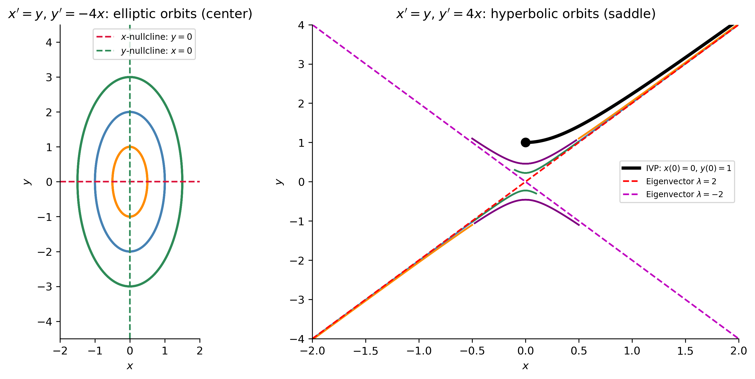
For \(x' = y\), \(y' = -4x\), the vector field is \(\mathbf{F}(x,y) = (y, -4x)\).

  • \(x\)-nullcline: \(y = 0\) (the \(x\)-axis), where the vectors point vertically.
  • \(y\)-nullcline: \(x = 0\) (the \(y\)-axis), where the vectors point horizontally.
  • Upper half-plane (\(y>0\)): \(x' > 0\), so \(x\) is increasing \(\Rightarrow\) motion to the right.
  • Right half-plane (\(x>0\)): \(y' < 0\), so \(y\) is decreasing \(\Rightarrow\) motion downward.

This gives the clockwise rotation visible in the phase-plane figure above.


Example 4.4 — Verifying a Solution and Finding the Orbit

Problem. Show that \(x(t) = \cos 2t\), \(y(t) = -2\sin 2t\) solves \(x' = y\), \(y' = -4x\).

Verification: \(x'(t) = -2\sin 2t = y(t)\) ✓; \(y'(t) = -4\cos 2t = -4x(t)\) ✓.

Finding the orbit. Compute \(x^2 + \frac{1}{4}y^2 = \cos^2 2t + \sin^2 2t = 1\).

So the orbit is the ellipse \(x^2 + \tfrac{1}{4}y^2 = 1\), traced clockwise with period \(\pi\).


The General Solution Structure

The example above reveals the form of the general solution to any linear system.

ImportantTheorem 4.8 — Superposition (Logan)

If \(\mathbf{x}_1(t)\) and \(\mathbf{x}_2(t)\) are any two vector solutions of the linear system (4.1)–(4.2), then \(\mathbf{x}(t) = c_1\mathbf{x}_1(t) + c_2\mathbf{x}_2(t)\) is a solution for any constants \(c_1\), \(c_2\).

ImportantTheorem 4.9 — Uniqueness (Logan)

The IVP \(x' = ax+by\), \(y' = cx+dy\), \(x(t_0) = x_0\), \(y(t_0) = y_0\) has a unique solution valid for \(-\infty < t < \infty\).

Consequence: two distinct orbits in the phase plane cannot intersect.

Two solutions \(\mathbf{x}_1(t) = (\phi_1(t), \phi_2(t))^T\) and \(\mathbf{x}_2(t) = (\psi_1(t), \psi_2(t))^T\) form a fundamental set if their Wronskian \[W(t) = \phi_1(t)\psi_2(t) - \phi_2(t)\psi_1(t) \neq 0 \quad \text{for all } t.\]

ImportantTheorem 4.10 — General Solution (Logan)

If \(\mathbf{x}_1(t)\) and \(\mathbf{x}_2(t)\) form a fundamental set of solutions, then the general solution is \[\mathbf{x}(t) = c_1\mathbf{x}_1(t) + c_2\mathbf{x}_2(t). \tag{4.14}\]


Method of Elimination

A linear system can always be converted back to a single second-order equation by eliminating one variable.

General formula. For the system \(x' = ax + by\), \(y' = cx + dy\), differentiating the first equation and substituting \(y'\) from the second gives: \[x'' - (a+d)x' + (ad - bc)x = 0. \tag{4.7}\] Once \(x(t)\) is found, \(y(t)\) is recovered from \[y(t) = \frac{1}{b}(x' - ax). \tag{4.8}\]

Note that the coefficients of (4.7) are: - \(-(a+d) = -\text{tr}(A)\) (negative trace of the coefficient matrix) - \((ad-bc) = \det(A)\) (determinant of the coefficient matrix)

These are the same quantities that appear in the characteristic equation \(\lambda^2 - \text{tr}(A)\lambda + \det(A) = 0\), which is no coincidence — we will return to this in Section 4.3.

NoteExample 4.6 (Logan) — Elimination

For \(x' = y\), \(y' = -4x\): differentiating the first gives \(x'' = y' = -4x\), so \[x'' + 4x = 0.\] General solution: \(x(t) = c_1\cos 2t + c_2\sin 2t\), \(y(t) = x' = -2c_1\sin 2t + 2c_2\cos 2t\).

In vector form: \[\mathbf{x}(t) = c_1\begin{pmatrix}\cos 2t \\ -2\sin 2t\end{pmatrix} + c_2\begin{pmatrix}\sin 2t \\ 2\cos 2t\end{pmatrix}.\]

Wronskian check: \(W = (\cos 2t)(2\cos 2t) - (-2\sin 2t)(\sin 2t) = 2\cos^2 2t + 2\sin^2 2t = 2 \neq 0\). \(\checkmark\)

NoteExample 4.12 (Logan) — Real Eigenvalues via Elimination

For \(x' = y\), \(y' = 4x\) (note the positive sign): differentiating gives \(x'' - 4x = 0\).

General solution: \(x(t) = c_1 e^{2t} + c_2 e^{-2t}\), \(y(t) = 2c_1 e^{2t} - 2c_2 e^{-2t}\).

\[\mathbf{x}(t) = c_1\begin{pmatrix}e^{2t}\\2e^{2t}\end{pmatrix} + c_2\begin{pmatrix}e^{-2t}\\-2e^{-2t}\end{pmatrix}.\]

Wronskian: \(W = e^{2t}(-2e^{-2t}) - 2e^{2t}(e^{-2t}) = -4 \neq 0\). \(\checkmark\)

IVP \(x(0)=0\), \(y(0)=1\): Solving \(c_1+c_2=0\), \(2c_1-2c_2=1\) gives \(c_1 = \tfrac{1}{4}\), \(c_2 = -\tfrac{1}{4}\).

Show the code
fig, axes = plt.subplots(1, 2, figsize=(11, 5))
t_long = np.linspace(0, 2*np.pi, 400)
t_saddle = np.linspace(0, 1.2, 300)

# --- System 1: x'=y, y'=-4x (ellipses) ---
def sys1(t, s): return [s[1], -4*s[0]]
for ic, color in [((1,0),'steelblue'),((0.5,0),'darkorange'),((1.5,0),'seagreen')]:
    sol = solve_ivp(sys1,(0,2*np.pi),list(ic),dense_output=True,max_step=0.01)
    t_p = np.linspace(0,2*np.pi,400)
    axes[0].plot(sol.sol(t_p)[0], sol.sol(t_p)[1], color=color, lw=2)

# Nullclines
axes[0].axhline(0, color='crimson',   lw=1.5, ls='--', label='$x$-nullcline: $y=0$')
axes[0].axvline(0, color='seagreen',  lw=1.5, ls='--', label='$y$-nullcline: $x=0$')
axes[0].set_xlim(-2,2); axes[0].set_ylim(-4.5,4.5)
axes[0].set_aspect('equal')
axes[0].set_xlabel('$x$'); axes[0].set_ylabel('$y$')
axes[0].set_title(r"$x'=y$, $y'=-4x$: elliptic orbits (center)")
axes[0].legend(fontsize=8)

# --- System 2: x'=y, y'=4x (saddle) ---
def sys2(t, s): return [s[1], 4*s[0]]
# Multiple ICs
for ic, color in [((0.1,0.3),'steelblue'),((0.5,1.1),'darkorange'),
                  ((-0.1,0.3),'seagreen'),((-0.5,1.1),'purple')]:
    for ic, color in [((0.1,0.3),'steelblue'),((0.5,1.1),'darkorange'),
                  ((-0.1,0.3),'seagreen'),((-0.5,1.1),'purple')]:
        for sign in [1, -1]:
          ic_s = (ic[0]*sign, ic[1]*sign)

          def stop_event(t, y):
              return 5.0 - np.max(np.abs(y))
          stop_event.terminal  = True
          stop_event.direction = -1

          sol = solve_ivp(sys2, (0, 1.5), list(ic_s),
                        dense_output=True, max_step=0.005,
                        events=stop_event)
          t_p = np.linspace(0, sol.t[-1], 200)
          axes[1].plot(sol.sol(t_p)[0], sol.sol(t_p)[1], color=color, lw=1.5)

# IVP solution c1=1/4, c2=-1/4
t_ivp = np.linspace(0,1.2,200)
x_ivp = 0.25*np.exp(2*t_ivp) - 0.25*np.exp(-2*t_ivp)
y_ivp = 0.5*np.exp(2*t_ivp) + 0.5*np.exp(-2*t_ivp)
axes[1].plot(x_ivp, y_ivp, 'k-', lw=3, label='IVP: $x(0)=0$, $y(0)=1$')
axes[1].plot(0, 1, 'ko', markersize=8, zorder=5)

# Eigenvectors (unstable/stable manifolds)
t_ev = np.linspace(-2,2,100)
axes[1].plot(t_ev, 2*t_ev, 'r--', lw=1.5, label='Eigenvector $\\lambda=2$')
axes[1].plot(t_ev,-2*t_ev, 'm--', lw=1.5, label='Eigenvector $\\lambda=-2$')
axes[1].set_xlim(-2,2); axes[1].set_ylim(-4,4)
axes[1].set_xlabel('$x$'); axes[1].set_ylabel('$y$')
axes[1].set_title(r"$x'=y$, $y'=4x$: hyperbolic orbits (saddle)")
axes[1].legend(fontsize=7.5)

plt.tight_layout(); plt.show()
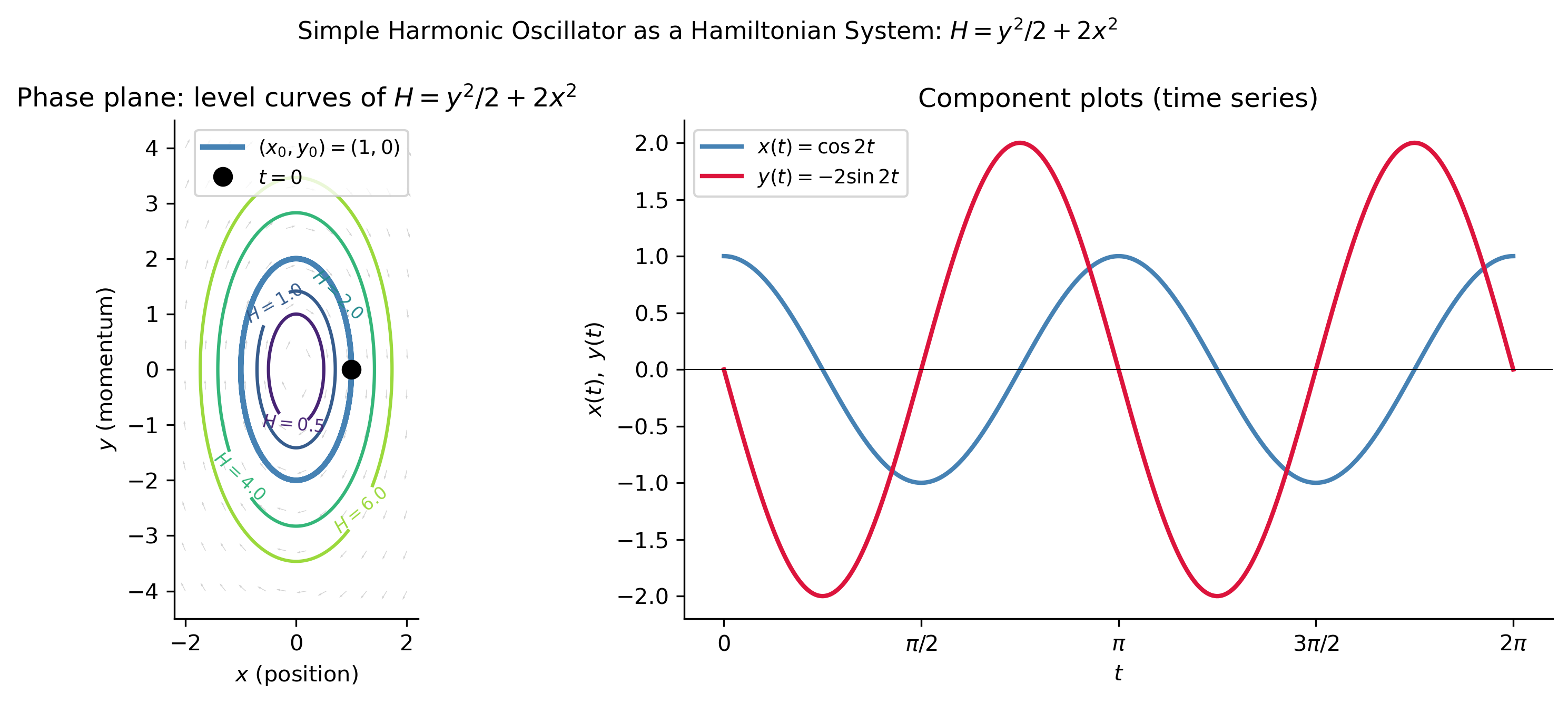
Figure 2: Phase-plane portraits and component plots for two systems solved by elimination. Left: \(x'=y\), \(y'=-4x\) — elliptic orbits (pure imaginary eigenvalues, neutral oscillation). Right: \(x'=y\), \(y'=4x\) — hyperbolic orbits (real eigenvalues, saddle point), with the IVP solution \(c_1=1/4\), \(c_2=-1/4\) highlighted.

The General Technique: \(n\)-th Order ODE to System

The reduction to a first-order system works for any order. For the \(n\)-th order linear ODE \[x^{(n)} + p_{n-1}x^{(n-1)} + \cdots + p_1 x' + p_0 x = 0,\] introduce the state variables \(x_1 = x\), \(x_2 = x'\), \(x_3 = x''\), \(\ldots\), \(x_n = x^{(n-1)}\). Then: \[\begin{cases} x_1' = x_2, \\ x_2' = x_3, \\ \quad\vdots \\ x_{n-1}' = x_n, \\ x_n' = -p_0 x_1 - p_1 x_2 - \cdots - p_{n-1}x_n. \end{cases}\]

In matrix form \(\mathbf{x}' = A\mathbf{x}\), where the companion matrix is:

\[A = \begin{pmatrix} 0 & 1 & 0 & \cdots & 0 \\ 0 & 0 & 1 & \cdots & 0 \\ \vdots & & & \ddots & \vdots \\ 0 & 0 & 0 & \cdots & 1 \\ -p_0 & -p_1 & -p_2 & \cdots & -p_{n-1} \end{pmatrix}.\]

The characteristic polynomial of \(A\) is exactly \(\lambda^n + p_{n-1}\lambda^{n-1} + \cdots + p_1\lambda + p_0 = 0\) — the same characteristic equation we solved in Chapter 2.

TipConnection to Notes 4

When \(n=2\) the companion matrix is \(A = \bigl[\begin{smallmatrix}0&1\\-c/a&-b/a\end{smallmatrix}\bigr]\), with characteristic equation \(\lambda^2 + (b/a)\lambda + (c/a) = 0\) — precisely equation (2.4) from Notes 4. The eigenvalues of the companion matrix are the roots of the ODE characteristic equation. This is the rigorous justification for the terminology “eigenvalues of a differential equation” used in Notes 4.

Show the code
print("2nd-order companion: x'' + (b/a)x' + (c/a)x = 0, y = x'")
a_v, b_v, c_v = 1, 3, 2  # x'' + 3x' + 2x = 0
A_2nd = sym.Matrix([[0,1],[-c_v/a_v, -b_v/a_v]])
lam = sym.Symbol('lambda')
char2 = (lam*sym.eye(2) - A_2nd).det()
print(f"  A = {A_2nd.tolist()}")
print(f"  char poly = {sym.expand(char2)}")
print(f"  eigenvalues = {sym.solve(char2, lam)}")

print("\n3rd-order companion: x''' + 2x'' - x' + 3x = 0")
A_3rd = sym.Matrix([[0,1,0],[0,0,1],[-3,1,-2]])
char3 = (lam*sym.eye(3) - A_3rd).det()
print(f"  char poly = {sym.expand(char3)}")
2nd-order companion: x'' + (b/a)x' + (c/a)x = 0, y = x'
  A = [[0, 1], [-2.00000000000000, -3.00000000000000]]
  char poly = lambda**2 + 3.0*lambda + 2.0
  eigenvalues = [-2.00000000000000, -1.00000000000000]

3rd-order companion: x''' + 2x'' - x' + 3x = 0
  char poly = lambda**3 + 2*lambda**2 - lambda + 3

Compartmental Model (Example 4.2, Logan)

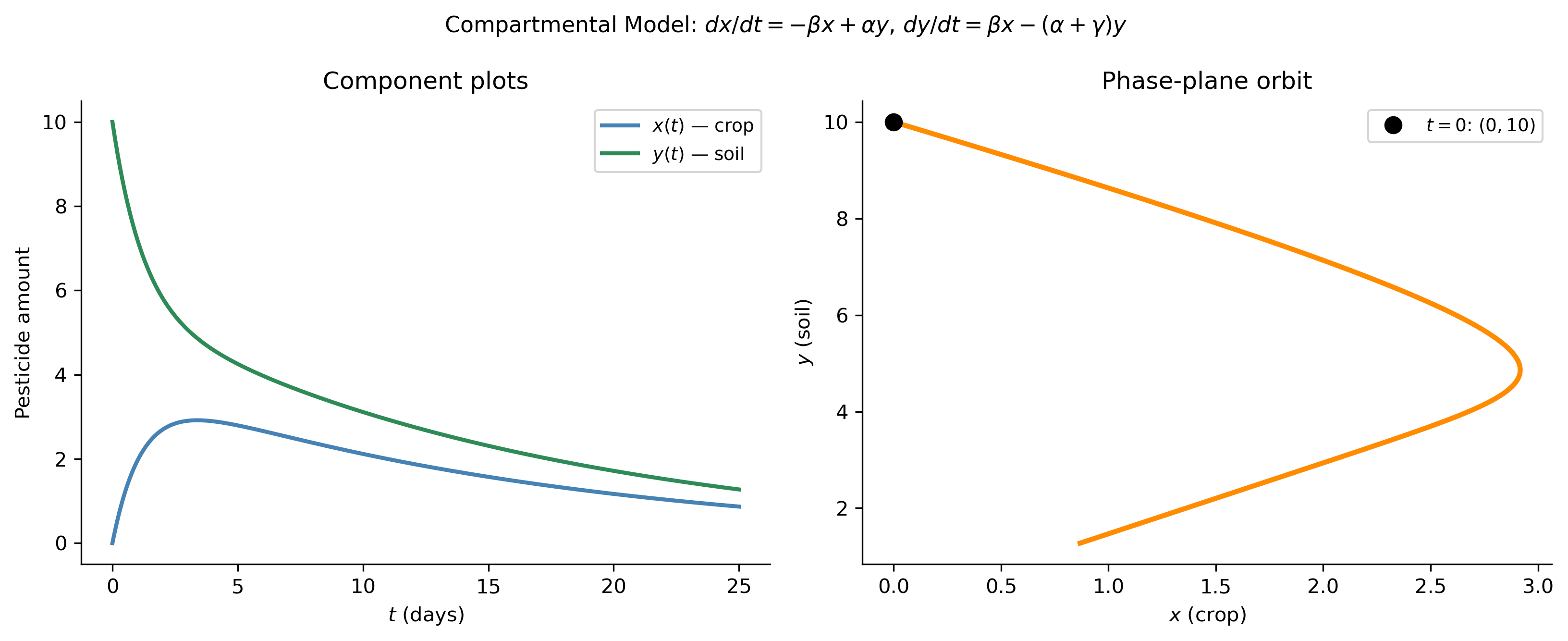
Many systems arise naturally as compartmental models — several interacting compartments exchanging material at prescribed rates. For a farm crop (amount \(x\)) and surrounding soil (amount \(y\)) with a pesticide:

\[\frac{dx}{dt} = -\beta x + \alpha y, \qquad \frac{dy}{dt} = \beta x - (\alpha+\gamma)y.\]

Here \(\alpha y\) is the uptake rate into the crop, \(\beta x\) the return rate to the soil, and \(\gamma y\) the natural degradation rate in the soil.

Show the code
alpha_v, beta_v, gamma_v = 0.3, 0.5, 0.1

def comp_sys(t, state):
    x_c, y_c = state
    return [-beta_v*x_c + alpha_v*y_c,
             beta_v*x_c - (alpha_v+gamma_v)*y_c]

t_eval = np.linspace(0, 25, 500)
sol_c = solve_ivp(comp_sys, (0,25), [0.0, 10.0], t_eval=t_eval, max_step=0.05)

fig, axes = plt.subplots(1, 2, figsize=(11, 4.5))
axes[0].plot(t_eval, sol_c.y[0], color='steelblue', lw=2, label='$x(t)$ — crop')
axes[0].plot(t_eval, sol_c.y[1], color='seagreen',  lw=2, label='$y(t)$ — soil')
axes[0].set_xlabel('$t$ (days)'); axes[0].set_ylabel('Pesticide amount')
axes[0].set_title('Component plots')
axes[0].legend(fontsize=9)

axes[1].plot(sol_c.y[0], sol_c.y[1], color='darkorange', lw=2.5)
axes[1].plot(0, 10, 'ko', markersize=8, label='$t=0$: $(0,10)$', zorder=5)
axes[1].set_xlabel('$x$ (crop)'); axes[1].set_ylabel('$y$ (soil)')
axes[1].set_title('Phase-plane orbit')
axes[1].legend(fontsize=9)

plt.suptitle(r'Compartmental Model: $dx/dt=-\beta x+\alpha y$, $dy/dt=\beta x-(\alpha+\gamma)y$', fontsize=11)
plt.tight_layout(); plt.show()
Figure 3: Compartmental pesticide model with \(\alpha=0.3\), \(\beta=0.5\), \(\gamma=0.1\), initial conditions \(x(0)=0\), \(y(0)=10\) (pesticide initially only in soil). The pesticide gradually transfers into the crop, reaches a peak, and both compartments eventually decay to zero as the pesticide degrades.

Other Approaches: Division and Laplace Transforms

Remark 4.14 (Division of equations): For simple systems, divide the two equations to obtain \(\frac{dy}{dx} = \frac{cx+dy}{ax+by}\), a first-order ODE for the orbit shape \(y = y(x)\) with \(t\) suppressed. For Example 4.3: \(dy/dx = -4x/y\), which separates to give \(x^2 + \tfrac{1}{4}y^2 = C\).

Remark 4.15 (Laplace transforms): Apply \(\mathcal{L}\) to each equation to obtain a \(2\times 2\) algebraic system for \(X(s) = \mathcal{L}[x]\) and \(Y(s) = \mathcal{L}[y]\): \[sX(s) - x(0) = aX(s) + bY(s), \qquad sY(s) - y(0) = cX(s) + dY(s).\] Solve for \(X(s)\), \(Y(s)\), then invert. Best for problems with discontinuous or impulsive forcing.


Part 2 — Section 4.2: Matrices and Linear Systems

Section 4.2.1 — Preliminaries from Algebra

A \(2\times 2\) matrix is a rectangular array of four real numbers: \[A = \begin{pmatrix} a_{11} & a_{12} \\ a_{21} & a_{22} \end{pmatrix}.\] The entry \(a_{ij}\) is in row \(i\), column \(j\). The main diagonal consists of \(a_{11}, a_{22}\). Matrices are denoted by uppercase letters; vectors (column matrices) by lowercase boldface: \[\mathbf{x} = \begin{pmatrix}x_1 \\ x_2\end{pmatrix}, \quad \text{written as } \mathbf{x} = (x_1,x_2)^T.\]

Arithmetic rules: - Addition (entrywise): \((A+B)_{ij} = a_{ij}+b_{ij}\). - Scalar multiplication: \((cA)_{ij} = ca_{ij}\). - Matrix product: \((AB)_{ij} = \sum_k a_{ik}b_{kj}\) (row \(i\) of \(A\) dotted with column \(j\) of \(B\)).

ImportantImportant: Matrix Multiplication is NOT Commutative

In general \(AB \neq BA\). Order matters. A concrete counterexample: \[A = \begin{pmatrix}1&1\\0&0\end{pmatrix}, \quad B = \begin{pmatrix}0&0\\1&1\end{pmatrix}.\] \[AB = \begin{pmatrix}1&1\\0&0\end{pmatrix}\begin{pmatrix}0&0\\1&1\end{pmatrix} = \begin{pmatrix}1&1\\0&0\end{pmatrix}, \qquad BA = \begin{pmatrix}0&0\\1&1\end{pmatrix}\begin{pmatrix}1&1\\0&0\end{pmatrix} = \begin{pmatrix}0&0\\1&1\end{pmatrix}.\] Since \(AB = A \neq B = BA\), these two products are different. (See the code block below for a SymPy check.)

Properties that do hold: - Associativity: \(A(BC) = (AB)C\). - Distributivity: \(A(B+C) = AB + AC\). - Identity: \(AI = IA = A\).

The Determinant and Inverse

The determinant of a \(2\times 2\) matrix is the scalar: \[\det A = \det\begin{pmatrix}a&b\\c&d\end{pmatrix} = ad - bc.\]

If \(\det A \neq 0\), \(A\) is nonsingular (invertible) and its inverse is: \[A^{-1} = \frac{1}{\det A}\begin{pmatrix}d & -b \\ -c & a\end{pmatrix}. \tag{4.17}\]

The recipe: swap the main diagonal, negate the off-diagonal, divide by \(\det A\).

NoteExample 4.18 (Logan)

For \(A = \bigl[\begin{smallmatrix}1&2\\4&3\end{smallmatrix}\bigr]\): \(\det A = 3 - 8 = -5\), so \[A^{-1} = \frac{1}{-5}\begin{pmatrix}3&-2\\-4&1\end{pmatrix} = \begin{pmatrix}-3/5 & 2/5 \\ 4/5 & -1/5\end{pmatrix}.\] Verify: \(AA^{-1} = I\). \(\checkmark\)

ImportantKey Result: \(A^{-1}\) exists \(\Longleftrightarrow\) \(\det A \neq 0\).
Show the code
print("=== Examples 4.16 and 4.17 (Logan) ===")
A = sym.Matrix([[1,2],[3,-4]]); B = sym.Matrix([[0,-2],[7,-4]])
x_v = sym.Matrix([-4,6]);      y_v = sym.Matrix([5,1])
print(f"A+B =\n{A+B}")
print(f"-3B =\n{-3*B}")
print(f"5x = {(5*x_v).T}")
print(f"x+2y = {(x_v+2*y_v).T}")

A2 = sym.Matrix([[2,3],[-1,0]]); B2 = sym.Matrix([[1,4],[5,2]])
print(f"\nAB =\n{A2*B2}")
print(f"A^2 =\n{A2**2}")

print("\n=== Non-commutativity: AB ≠ BA ===")
Anc = sym.Matrix([[1,1],[0,0]]); Bnc = sym.Matrix([[0,0],[1,1]])
print(f"A =\n{Anc}\nB =\n{Bnc}")
print(f"AB =\n{Anc*Bnc}")
print(f"BA =\n{Bnc*Anc}")
print(f"AB == BA? {Anc*Bnc == Bnc*Anc}")

print("\n=== Example 4.18 ===")
A18 = sym.Matrix([[1,2],[4,3]])
print(f"det(A) = {A18.det()},  A^(-1) =\n{A18.inv()}")
print(f"A*A^(-1) = {A18*A18.inv()}")
=== Examples 4.16 and 4.17 (Logan) ===
A+B =
Matrix([[1, 0], [10, -8]])
-3B =
Matrix([[0, 6], [-21, 12]])
5x = Matrix([[-20, 30]])
x+2y = Matrix([[6, 8]])

AB =
Matrix([[17, 14], [-1, -4]])
A^2 =
Matrix([[1, 6], [-2, -3]])

=== Non-commutativity: AB ≠ BA ===
A =
Matrix([[1, 1], [0, 0]])
B =
Matrix([[0, 0], [1, 1]])
AB =
Matrix([[1, 1], [0, 0]])
BA =
Matrix([[0, 0], [1, 1]])
AB == BA? False

=== Example 4.18 ===
det(A) = -5,  A^(-1) =
Matrix([[-3/5, 2/5], [4/5, -1/5]])
A*A^(-1) = Matrix([[1, 0], [0, 1]])

Matrix-Vector Product

\[A\mathbf{x} = \begin{pmatrix}a&b\\c&d\end{pmatrix}\begin{pmatrix}x\\y\end{pmatrix} = \begin{pmatrix}ax+by\\cx+dy\end{pmatrix}.\]

This is the key operation connecting matrices to systems of equations. Note: \(\mathbf{x}A\) (vector on the left) is not defined for column vectors.

Systems of Algebraic Equations

The system \(a_{11}x_1 + a_{12}x_2 = b_1\), \(a_{21}x_1 + a_{22}x_2 = b_2\) is written compactly as: \[A\mathbf{x} = \mathbf{b}. \tag{4.18}\]

ImportantTheorem 4.19 (Logan)
  1. If \(\det A \neq 0\): the system \(A\mathbf{x}=\mathbf{b}\) has the unique solution \(\mathbf{x} = A^{-1}\mathbf{b}\); the homogeneous system \(A\mathbf{x}=\mathbf{0}\) has only \(\mathbf{x}=\mathbf{0}\).
  2. If \(\det A = 0\): \(A\mathbf{x}=\mathbf{0}\) has infinitely many solutions; \(A\mathbf{x}=\mathbf{b}\) has no solution or infinitely many.

Cramer’s Rule

ImportantTheorem 4.21 — Cramer’s Rule (Logan)

The solution to \(A\mathbf{x} = \mathbf{b}\) (when \(\det A \neq 0\)) is: \[x_1 = \frac{\det\begin{pmatrix}b_1 & a_{12} \\ b_2 & a_{22}\end{pmatrix}}{\det A}, \qquad x_2 = \frac{\det\begin{pmatrix}a_{11} & b_1 \\ a_{21} & b_2\end{pmatrix}}{\det A}.\] Replace column \(j\) of \(A\) with \(\mathbf{b}\) to get the numerator determinant for \(x_j\).

NoteExample 4.22 (Logan)

Solve \(2x-3y=4\), \(4x-y=-1\).

\(\det A = (2)(-1)-(4)(-3) = 10\).

\[x = \frac{\det\bigl[\begin{smallmatrix}4&-3\\-1&-1\end{smallmatrix}\bigr]}{10} = \frac{-7}{10}, \qquad y = \frac{\det\bigl[\begin{smallmatrix}2&4\\4&-1\end{smallmatrix}\bigr]}{10} = \frac{-18}{10} = -\frac{9}{5}.\]

Linear Independence and the Nullspace

Two vectors \(\mathbf{v}, \mathbf{w}\) are linearly independent if the only solution to \(c_1\mathbf{v} + c_2\mathbf{w} = \mathbf{0}\) is \(c_1 = c_2 = 0\). This is equivalent to: \[\det\begin{pmatrix}v_1 & w_1 \\ v_2 & w_2\end{pmatrix} \neq 0. \tag{4.19}\]

The nullspace of \(A\) is the set of all solutions to \(A\mathbf{x}=\mathbf{0}\): - \(\det A \neq 0\): nullspace = \(\{\mathbf{0}\}\) (only the trivial solution). - \(\det A = 0\): nullspace = a line through the origin.

Show the code
print("=== Example 4.20 (Logan): singular matrix ===")
A20 = sym.Matrix([[4,1],[8,2]])
print(f"det(A) = {A20.det()} (singular)")
print(f"Nullspace: {A20.nullspace()}")
print(f"All solutions: x = alpha*(1,-4)^T for alpha in R")

print("\n=== Example 4.22 (Logan): Cramer's rule ===")
A22 = sym.Matrix([[2,-3],[4,-1]]); b22 = sym.Matrix([4,-1])
print(f"det(A) = {A22.det()}")
A_x = sym.Matrix([[4,-3],[-1,-1]]); A_y = sym.Matrix([[2,4],[4,-1]])
x_cr = A_x.det()/A22.det(); y_cr = A_y.det()/A22.det()
print(f"x = {x_cr}, y = {y_cr}")
print(f"Verify: 2x-3y = {2*x_cr - 3*y_cr}, 4x-y = {4*x_cr - y_cr}")
=== Example 4.20 (Logan): singular matrix ===
det(A) = 0 (singular)
Nullspace: [Matrix([
[-1/4],
[   1]])]
All solutions: x = alpha*(1,-4)^T for alpha in R

=== Example 4.22 (Logan): Cramer's rule ===
det(A) = 10
x = -7/10, y = -9/5
Verify: 2x-3y = 4, 4x-y = -1

Section 4.2.2 — The Matrix Form \(\mathbf{x}' = A\mathbf{x}\)

The system (4.1)–(4.2) is written compactly as: \[\mathbf{x}'(t) = A\mathbf{x}(t), \tag{4.22}\] where \[\mathbf{x}(t) = \begin{pmatrix}x(t)\\y(t)\end{pmatrix}, \quad A = \begin{pmatrix}a&b\\c&d\end{pmatrix}, \quad \mathbf{x}'(t) = \begin{pmatrix}x'(t)\\y'(t)\end{pmatrix}.\]

Since the right-hand side does not depend explicitly on \(t\), the system is autonomous.

Equilibria and Critical Points

An equilibrium solution of \(\mathbf{x}' = A\mathbf{x}\) is a constant vector \(\mathbf{x}^*\) satisfying \[A\mathbf{x}^* = \mathbf{0}.\] In the phase plane, \(\mathbf{x}^*\) plots as a single point — a critical point.

ImportantTheorem 4.23 (Logan)

The linear system \(\mathbf{x}' = A\mathbf{x}\) has: 1. A unique equilibrium at \((0,0)\) if \(\det A \neq 0\). 2. A straight line of equilibria (nonisolated) if \(\det A = 0\).

Stability

For an isolated critical point at \((0,0)\):

  • Asymptotically stable (attractor/sink): nearby orbits converge to \((0,0)\) as \(t\to+\infty\).
  • Stable (neutrally stable/center): nearby orbits remain nearby but need not converge.
  • Unstable (repeller/source): it is not stable — some nearby orbits move away.

Nonhomogeneous Systems and Remark 4.24

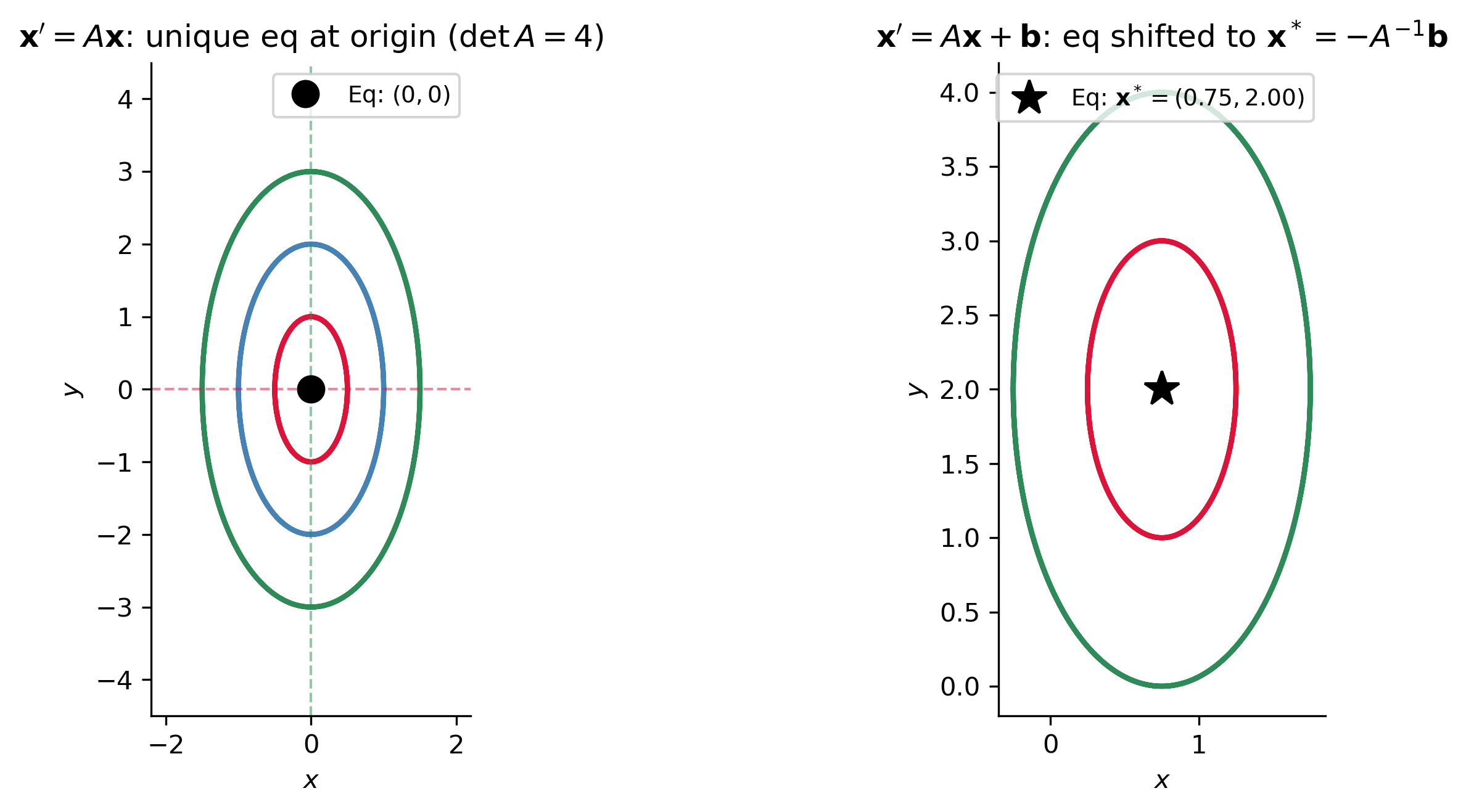
For the nonhomogeneous system \[\mathbf{x}' = A\mathbf{x} + \mathbf{b}, \quad \det A \neq 0, \tag{4.23}\] the unique critical point is found by setting \(\mathbf{x}' = \mathbf{0}\): \[\mathbf{x}^* = -A^{-1}\mathbf{b}. \tag{4.24}\]

Reduction to homogeneous form: let \(\mathbf{y} = \mathbf{x} - \mathbf{x}^*\). Then \(\mathbf{y}' = \mathbf{x}' = A(\mathbf{y}+\mathbf{x}^*) + \mathbf{b} = A\mathbf{y}\). So analyzing \(\mathbf{x}' = A\mathbf{x}+\mathbf{b}\) reduces to analyzing \(\mathbf{y}' = A\mathbf{y}\), centered at the new origin \(\mathbf{x}^*\).

Show the code
fig, axes = plt.subplots(1, 2, figsize=(11, 4.5))

# System 1: x'=Ax, A=[[0,1],[-4,0]], unique eq at origin
def sys_center(t,s): return [s[1], -4*s[0]]
for ic, color in [((1,0),'steelblue'),((0.5,0),'darkorange'),((1.5,0),'seagreen'),
                  ((0,1),'crimson')]:
    sol = solve_ivp(sys_center,(0,2*np.pi),list(ic),dense_output=True,max_step=0.01)
    t_p = np.linspace(0,2*np.pi,400)
    axes[0].plot(sol.sol(t_p)[0],sol.sol(t_p)[1],color=color,lw=2)
axes[0].plot(0,0,'ko',markersize=10,zorder=5,label='Eq: $(0,0)$')
axes[0].axhline(0,color='crimson',lw=1,ls='--',alpha=0.5)
axes[0].axvline(0,color='seagreen',lw=1,ls='--',alpha=0.5)
axes[0].set_aspect('equal'); axes[0].set_xlim(-2.2,2.2); axes[0].set_ylim(-4.5,4.5)
axes[0].set_xlabel('$x$'); axes[0].set_ylabel('$y$')
axes[0].set_title(r"$\mathbf{x}'=A\mathbf{x}$: unique eq at origin ($\det A=4$)")
axes[0].legend(fontsize=9)

# System 2: x'=Ax+b, equilibrium shifted
A_nh = np.array([[0,1],[-4,0]]); b_nh = np.array([-2.0,3.0])
x_star = -np.linalg.inv(A_nh)@b_nh
print(f"x* = -A^(-1)b = {x_star}")

def sys_nh(t,s):
    return [A_nh[0,0]*s[0]+A_nh[0,1]*s[1]+b_nh[0],
            A_nh[1,0]*s[0]+A_nh[1,1]*s[1]+b_nh[1]]
for ic_offset, color in [(np.array([1,0]),'steelblue'),(np.array([0.5,0]),'darkorange'),
                          (np.array([-1,0]),'seagreen'),(np.array([0,1]),'crimson')]:
    ic = x_star + ic_offset
    sol = solve_ivp(sys_nh,(0,2*np.pi),list(ic),dense_output=True,max_step=0.01)
    t_p = np.linspace(0,2*np.pi,400)
    axes[1].plot(sol.sol(t_p)[0],sol.sol(t_p)[1],color=color,lw=2)
axes[1].plot(*x_star,'k*',markersize=14,zorder=5,label=f'Eq: $\\mathbf{{x}}^*=({x_star[0]:.2f},{x_star[1]:.2f})$')
axes[1].set_aspect('equal')
axes[1].set_xlabel('$x$'); axes[1].set_ylabel('$y$')
axes[1].set_title(r"$\mathbf{x}'=A\mathbf{x}+\mathbf{b}$: eq shifted to $\mathbf{x}^*=-A^{-1}\mathbf{b}$")
axes[1].legend(fontsize=9)

plt.tight_layout(); plt.show()
x* = -A^(-1)b = [0.75 2.  ]
Figure 4: Equilibria of two systems. Left: \(\mathbf{x}'=A\mathbf{x}\) with \(A=\bigl[\begin{smallmatrix}0&1\\-4&0\end{smallmatrix}\bigr]\), \(\det A=4\neq 0\) — unique isolated equilibrium at origin (stable center). Right: \(\mathbf{x}'=A\mathbf{x}+\mathbf{b}\) with \(\mathbf{b}=(-2,3)^T\) — the equilibrium shifts to \(\mathbf{x}^*=-A^{-1}\mathbf{b}\).

Summary

Concept Formula / Rule Section
Second-order to system \(y=x'\): \(x'=y\), \(y'=-(c/a)x-(b/a)y\) 4.1
Hamiltonian system \(\dot{q}=\partial H/\partial p\), \(\dot{p}=-\partial H/\partial q\) 4.1
\(n\)-th order companion State \((x_1,\ldots,x_n)=(x,x',\ldots,x^{(n-1)})\) 4.1
Elimination formula \(x''-(a+d)x'+(ad-bc)x=0\) 4.1 (4.7)
Wronskian \(W=\phi_1\psi_2-\phi_2\psi_1\neq 0\) 4.1
General solution \(\mathbf{x}=c_1\mathbf{x}_1+c_2\mathbf{x}_2\) Thm 4.10
Matrix inverse (\(2\times2\)) \(A^{-1}=\frac{1}{\det A}\bigl[\begin{smallmatrix}d&-b\\-c&a\end{smallmatrix}\bigr]\) 4.2 (4.17)
Unique solution iff \(\det A \neq 0\) Thm 4.19
Cramer’s rule Replace column with \(\mathbf{b}\), divide by \(\det A\) Thm 4.21
Matrix ODE \(\mathbf{x}'=A\mathbf{x}\) 4.2 (4.22)
Equilibrium \(A\mathbf{x}^*=\mathbf{0}\) (homog.) or \(\mathbf{x}^*=-A^{-1}\mathbf{b}\) (non-homog.) Thm 4.23, Rem 4.24

These notes are also viewable as a slide deck presentation: Open slides in full screen

Note

Next: Eigenvalues and solving linear systems — Logan §4.3 & 4.4.


Relevant Videos

Linear algebra in seven minutes:

Matrices top 10 must know:

Matrix systems of ODEs:

References

Logan, J David. 2015. A First Course in Differential Equations, Third Edition.
Show the code
import sys
print("Python:", sys.version)
print('\n'.join(f'{m.__name__}=={m.__version__}' for m in globals().values() if getattr(m,'__version__',None)))
Python: 3.14.4 | packaged by conda-forge | (main, Apr  8 2026, 02:33:53) [Clang 20.1.8 ]
numpy==2.4.3
sympy==1.14.0
matplotlib==3.10.8

Reuse

CC BY-NC-SA 4.0