\[\boxed{\text{ODE in } x(t)}
\;\xrightarrow{\;\mathcal{L}\;}\;
\boxed{\text{Algebraic equation in } X(s)}
\;\xrightarrow{\;\text{solve}\;}\;
\boxed{X(s)}
\;\xrightarrow{\;\mathcal{L}^{-1}\;}\;
\boxed{x(t)}\]
Transform: apply \(\mathcal{L}\) to both sides, using the derivative formulas and linearity.
Solve: the result is an algebraic equation for \(X(s)\). Solve it.
Invert: find \(x(t) = \mathcal{L}^{-1}[X(s)]\) using the table and partial fractions.
The initial conditions \(x(0)\) and \(x'(0)\) enter automatically in Step 1 — they are part of the derivative formula, not a separate enforcement step. This is one of the major advantages of the method.
The Derivative Formulas (Theorem 3.11)
The operational formulas that make the method work are:
Each formula has a clean structure: - The highest power of \(s\) times \(X(s)\). - Minus terms involving initial conditions with decreasing powers of \(s\).
For \(x'\): one factor of \(s\), one IC. For \(x''\): two factors of \(s\), two ICs. For \(x^{(n)}\): \(n\) factors, \(n\) ICs. The pattern generalizes directly.
Using the Derivative Formulas to Find Transforms
The formulas can also be used to find transforms of new functions without computing the defining integral.
Example 3.12 (Logan) — \(\mathcal{L}[t^2]\).
Notice that \((t^2)' = 2t\), so \(\mathcal{L}[(t^2)'] = \mathcal{L}[2t] = 2/s^2\). By (3.6) with \(x(0) = 0\): \[s\,\mathcal{L}[t^2] = \frac{2}{s^2} \;\Longrightarrow\; \mathcal{L}[t^2] = \frac{2}{s^3}.\]
Continuing by induction: \(\mathcal{L}[t^n] = n!/s^{n+1}\) for \(n = 0, 1, 2, 3, \ldots\)
Example 3.13 (Logan) — \(\mathcal{L}[\cosh t]\).
Using the identity \((\cosh t)'' = \cosh t\) and (3.7) with \(\cosh(0) = 1\), \(\sinh(0) = 0\): \[\mathcal{L}[\cosh t] = s^2\mathcal{L}[\cosh t] - s \;\Longrightarrow\; (1-s^2)\mathcal{L}[\cosh t] = -s \;\Longrightarrow\; \mathcal{L}[\cosh t] = \frac{s}{s^2-1}. \;\square\]
Step 3 — Invert. Checking the table: this matches the entry \(\dfrac{1}{(s-a)(s-b)} = \mathcal{L}\!\left[\dfrac{e^{at}-e^{bt}}{a-b}\right]\) with \(a=-1\), \(b=-2\): \[x(t) = \frac{e^{-t}-e^{-2t}}{-1-(-2)} = e^{-t} - e^{-2t}. \;\square\]
NoteExample 3.16 — Partial Fractions Verification
The table entry for \(1/[(s+1)(s+2)]\) may not always be immediately recognizable. Expanding in partial fractions confirms the result: \[\frac{1}{(s+1)(s+2)} = \frac{a}{s+1}+\frac{b}{s+2}.\] Clearing denominators: \(a(s+2) + b(s+1) = 1\). Equating coefficients: \(a+b=0\) and \(2a+b=1\), so \(a=1\), \(b=-1\). \[X(s) = \frac{1}{s+1} - \frac{1}{s+2} \;\Longrightarrow\; x(t) = e^{-t} - e^{-2t}. \;\checkmark\]
Inverting Transforms with Complex Poles — Completing the Square
Partial fractions for distinct real poles and repeated poles were introduced in Notes 6 (Types 1 and 2 of the inverse transform section). The examples above have already used those cases. Here we complete the picture with Type 3 — complex conjugate poles, which requires the additional technique of completing the square. Taken together, the three pole types cover every rational \(X(s)\) that arises from a constant-coefficient linear ODE.
Example 3.17 (Logan) — \(X(s) = 1/(s^2+3s+6)\).
Complete the square in the denominator: \[s^2+3s+6 = \left(s+\frac{3}{2}\right)^2 - \frac{9}{4} + 6 = \left(s+\frac{3}{2}\right)^2 + \left(\frac{\sqrt{15}}{2}\right)^2.\]
Now recognize the table form \(k/[(s-\alpha)^2+k^2]\) with \(\alpha = -3/2\) and \(k = \sqrt{15}/2\). Multiply and divide by \(\sqrt{15}/2\):
For \(s^2 + bs + c\) with \(4c > b^2\) (complex roots): \[s^2+bs+c = \left(s+\frac{b}{2}\right)^2 + \underbrace{\left(c - \frac{b^2}{4}\right)}_{\beta^2 > 0}.\] Then \(\alpha = -b/2\) and \(\beta = \sqrt{c - b^2/4}\).
Numerator adjustments: if the numerator is \(As + B\), rewrite it as \[A\left(s+\frac{b}{2}\right) + \left(B - \frac{Ab}{2}\right)\] and split into \(A\cdot\dfrac{s-\alpha}{(s-\alpha)^2+\beta^2}\) plus a multiple of \(\dfrac{\beta}{(s-\alpha)^2+\beta^2}\).
Step 1 — Transform. Apply \(\mathcal{L}\) to both sides. Using (3.7) and substituting the initial conditions explicitly: \[\bigl[s^2X(s) - s\cdot\underbrace{x(0)}_{=\,0} - \underbrace{x'(0)}_{=\,1}\bigr] - 2\bigl[sX(s) - \underbrace{x(0)}_{=\,0}\bigr] + 2X(s) = 0.\] The \(x(0) = 0\) terms vanish, and \(x'(0) = 1\) contributes \(-1\) on the left. Collecting \(X(s)\) terms: \[(s^2 - 2s + 2)X(s) = 1.\]
TipCommon Mistake to Avoid
A frequent error is to transform \(x'' - 2x' + 2x = 0\) and write \[s^2X - 2sX + 2X = 0 \quad \leftarrow \text{wrong when } x'(0)\neq 0\] forgetting that formula (3.7) contributes the initial condition terms \(-sx(0) - x'(0)\). With \(x(0)=0\) and \(x'(0)=1\), the correct left side picks up a \(-1\) from the \(-x'(0)\) term. Writing the unsimplified form first — as shown above — is a reliable way to avoid dropping ICs.
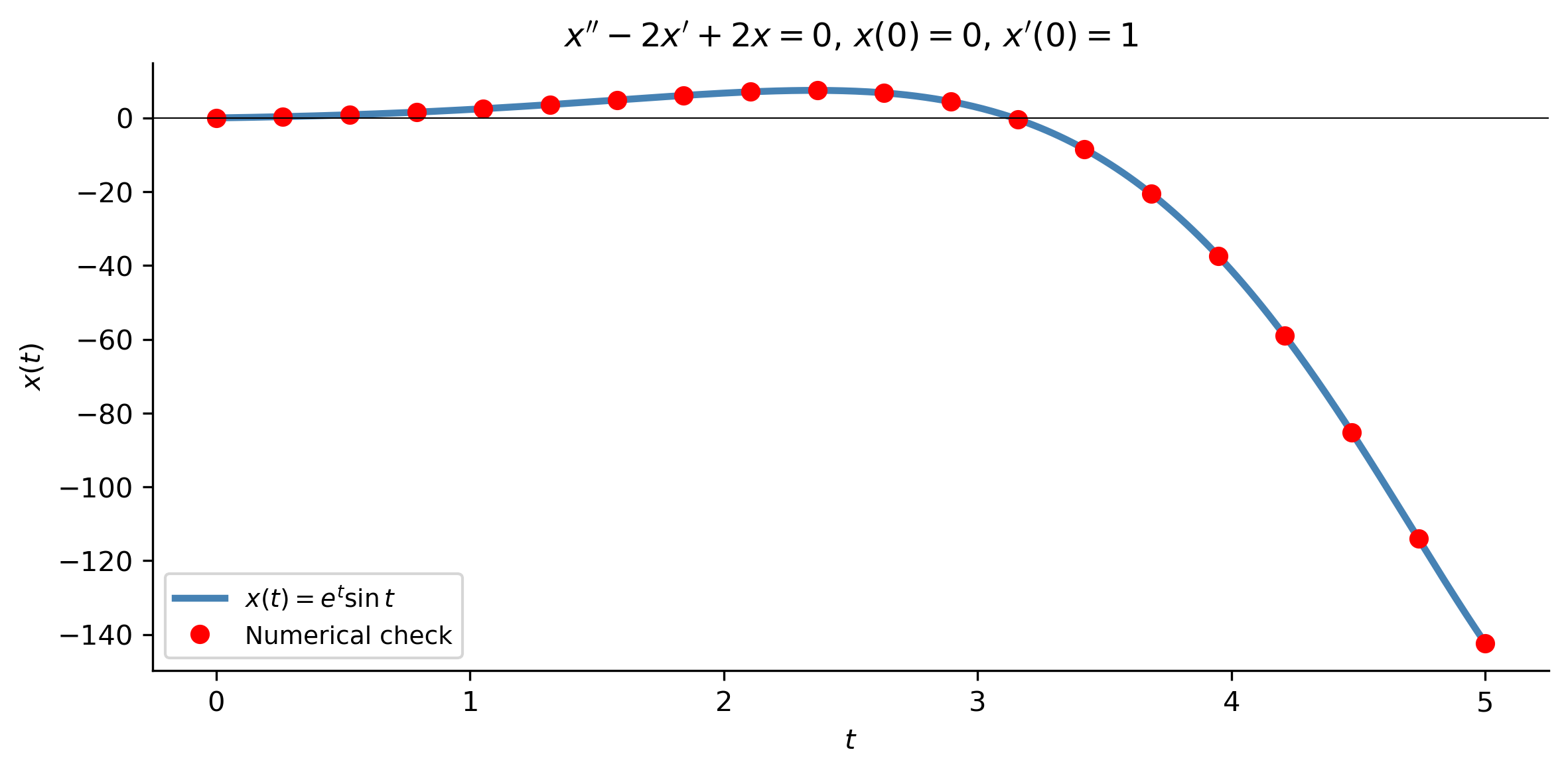
Step 2 — Solve:\[X(s) = \frac{1}{s^2-2s+2}.\]
Step 3 — Complete the square:\(s^2-2s+2 = (s-1)^2+1\).
Figure 1: Solution of \(x''-2x'+2x=0\), \(x(0)=0\), \(x'(0)=1\). The factor \(e^t\) causes the amplitude to grow while \(\sin t\) provides the oscillation. Red dots confirm the Laplace transform result against a direct numerical solve.
Nonhomogeneous Equation with Three-Term Partial Fractions
Step 1 — Transform. Apply \(\mathcal{L}\) to both sides, using the derivative formulas with \(x(0)=x'(0)=0\): \[(s^2+3s+2)X(s) = \mathcal{L}[e^t] = \frac{1}{s-1}.\]
One of the major reasons to use the Laplace transform is its ability to handle piecewise continuous (PWC) forcing without case-by-case analysis. Without Laplace transforms we would need to solve the ODE on each sub-interval separately, then match solutions at each junction — a tedious task. The Laplace transform handles everything in a single calculation.
Writing Piecewise Functions with Heaviside Steps
Recall from Notes 6 that any piecewise function can be written as a sum of Heaviside steps. The formula for a function that switches between expressions is: \[f(t) = f_1(t) + [f_2(t)-f_1(t)]\,H(t-a) + [f_3(t)-f_2(t)]\,H(t-b) + \cdots\]
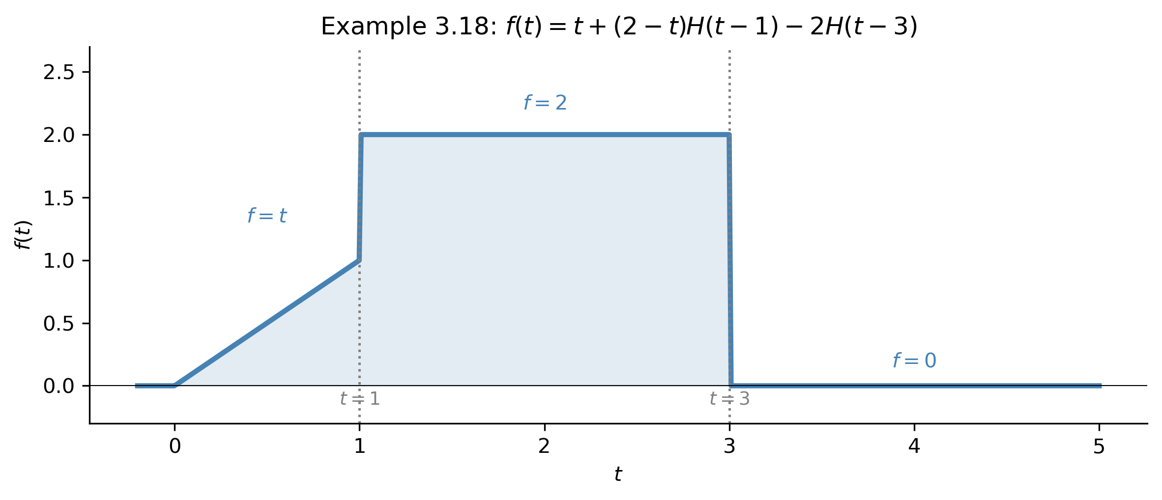
Example 3.18 (Logan). Express and transform \[f(t) = \begin{cases} t, & 0 < t < 1 \\ 2, & 1 \leq t \leq 3 \\ 0, & t > 3 \end{cases}\]
Heaviside form:\(f(t) = t + (2-t)H(t-1) - 2H(t-3)\).
To transform \(\mathcal{L}[tH(t-1)]\), use the table entry \(\mathcal{L}[f(t)H(t-a)] = e^{-as}\mathcal{L}[f(t+a)]\) with \(f(t)=t\): \[\mathcal{L}[tH(t-1)] = e^{-s}\mathcal{L}[t+1] = e^{-s}\!\left(\frac{1}{s^2}+\frac{1}{s}\right).\]
Figure 2: The piecewise function from Example 3.18: \(f(t)=t\) for \(0<t<1\), then \(f(t)=2\) for \(1\leq t\leq 3\), then \(f(t)=0\) for \(t>3\), expressed as \(t+(2-t)H(t-1)-2H(t-3)\).
Example 3.19 — Oscillator with One-Hump Sine Forcing
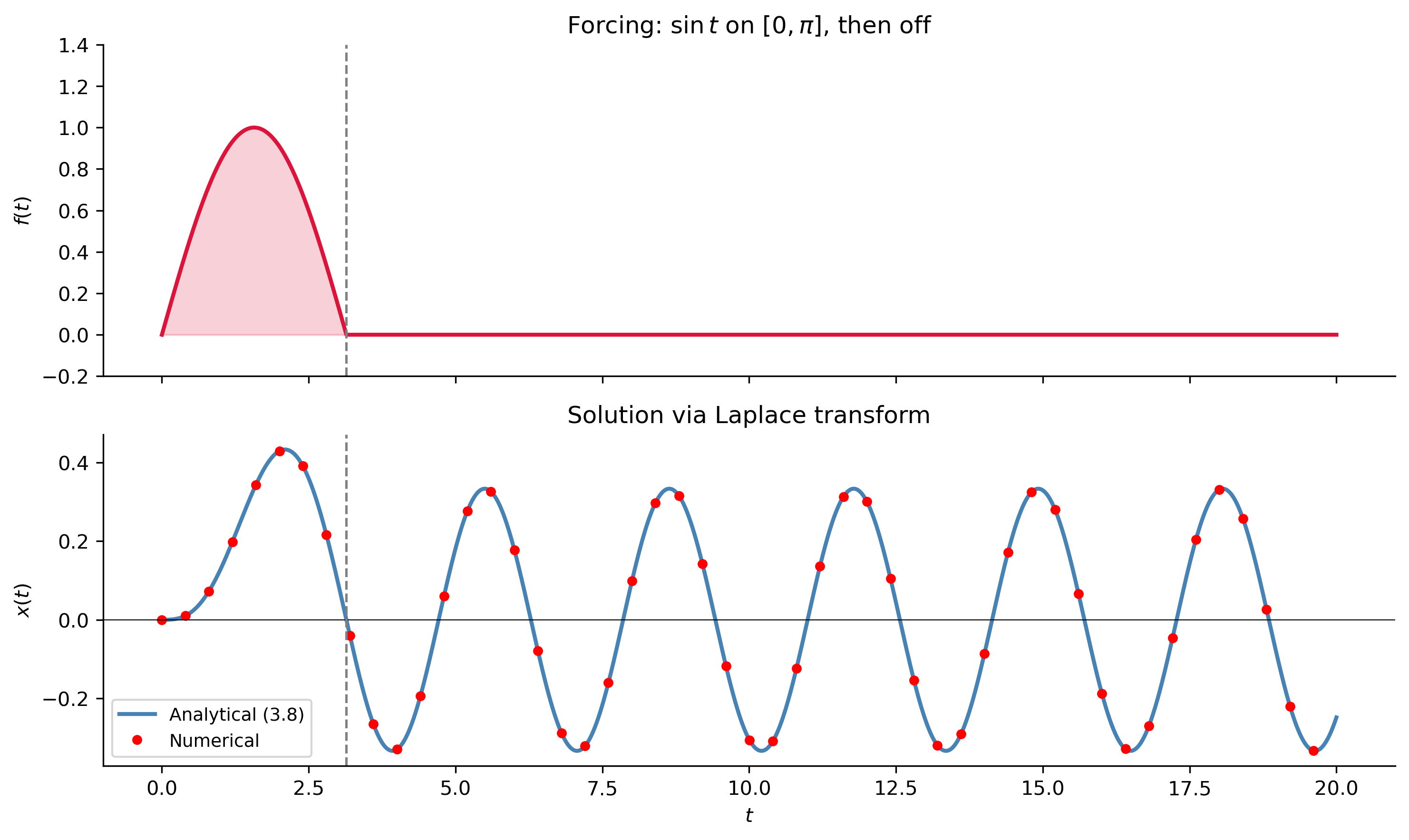
Figure 3: Example 3.19: \(x''+4x = \sin t - H(t-\pi)\sin t\), \(x(0)=x'(0)=0\). The forcing (top) is one arch of \(\sin t\) on \([0,\pi]\), then zero. After the forcing turns off at \(t=\pi\) the oscillator continues with a modified amplitude and phase — the free oscillation driven by the residual energy stored during \([0,\pi]\).
Example 3.21 — RC Circuit with Square-Pulse Forcing
Step 3 — Invert. By partial fractions: \(\dfrac{1}{s(s+3)} = \dfrac{1/3}{s} - \dfrac{1/3}{s+3}\), so \[\mathcal{L}^{-1}\!\left[\frac{1}{s(s+3)}\right] = \frac{1}{3}(1-e^{-3t}).\]
Apply the switching property to each term: \[\mathcal{L}^{-1}\!\left[\frac{e^{-s}}{s(s+3)}\right] = \frac{1}{3}(1-e^{-3(t-1)})H(t-1), \qquad
\mathcal{L}^{-1}\!\left[\frac{e^{-2s}}{s(s+3)}\right] = \frac{1}{3}(1-e^{-3(t-2)})H(t-2).\]
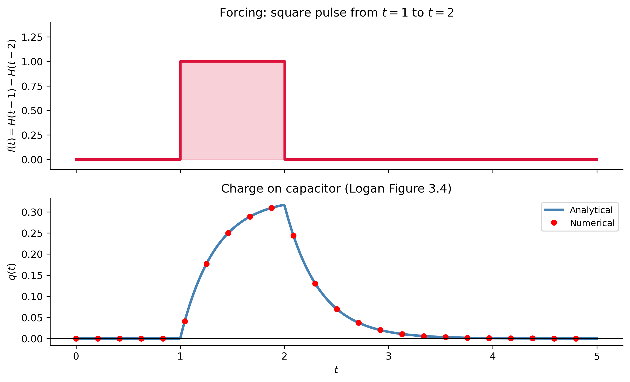
Figure 4: Example 3.21 (Logan, Figure 3.4): RC circuit charge \(q(t)\) under a square-pulse voltage. The switch opens at \(t=0\) (zero current), closes at \(t=1\) (charge builds), opens again at \(t=2\) (charge decays). The solution consists of two Heaviside-shifted exponential charging/discharging curves.
Remark 3.20 — Smoothing by Integration
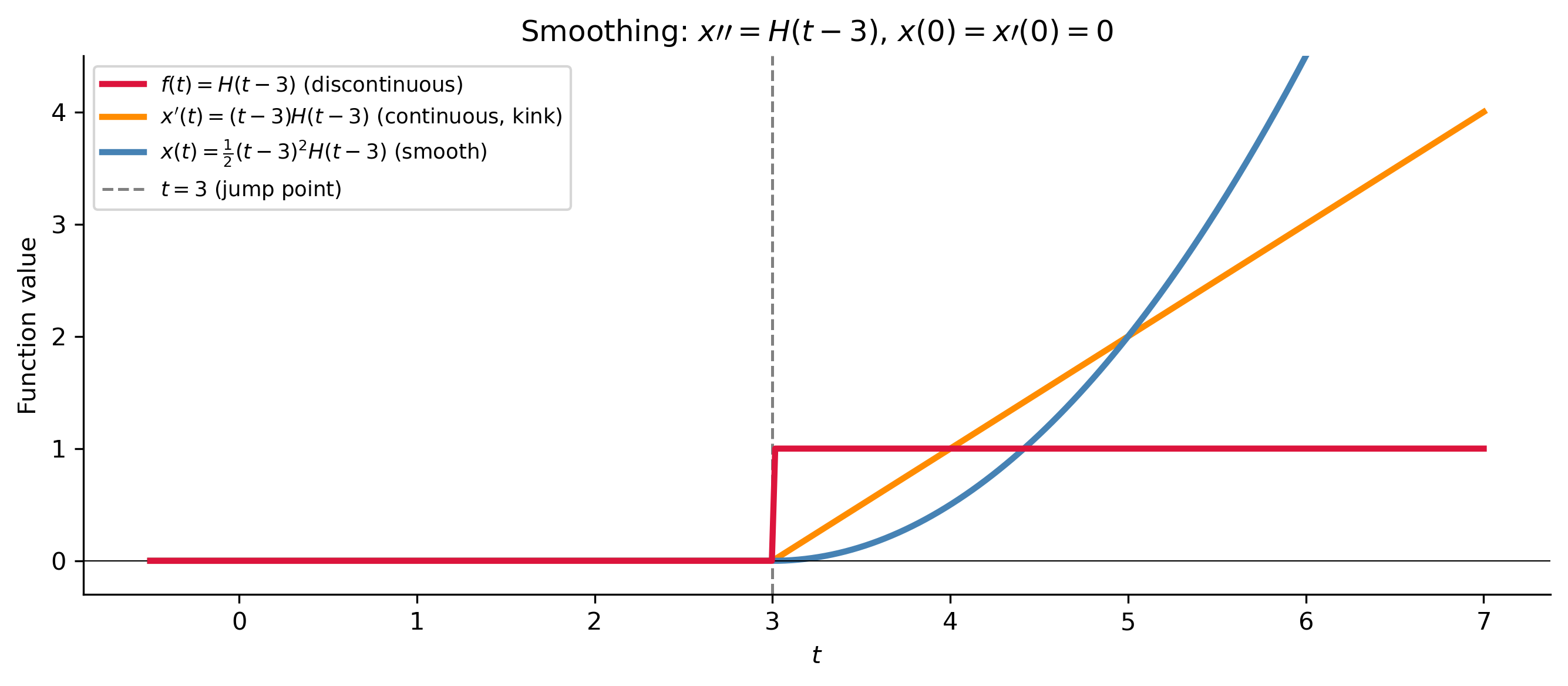
When the input \(f(t)\) of an ODE is only piecewise continuous, it is natural to ask: what regularity does the solution \(x(t)\) possess?
If \(f(t)\) is PWC and \(ax'' + bx' + cx = f(t)\), then the solution \(x(t)\) is continuous — and in fact continuously differentiable — even at points where \(f\) jumps. Integration is a smoothing operation: each time we integrate a function, we gain one degree of regularity.
Illustration. Consider \(x'' = H(t-3)\), \(x(0)=x'(0)=0\), where \(f(t)=H(t-3)\) has a jump at \(t=3\).
Integrating once: \(x'(t) = \displaystyle\int H(t-3)\,dt = (t-3)H(t-3)\). This is continuous (no jump), but its derivative has a jump at \(t=3\).
Integrating again: \(x(t) = \dfrac{1}{2}(t-3)^2 H(t-3)\). This is continuously differentiable.
Figure 5: Smoothing by integration (Remark 3.20). The Heaviside input \(f(t)=H(t-3)\) (red, discontinuous at \(t=3\)) produces a continuous but only piecewise-smooth \(x'(t)=(t-3)H(t-3)\) (orange, kink at \(t=3\)), and a smoothly differentiable solution \(x(t)=\frac{1}{2}(t-3)^2H(t-3)\) (blue, parabola starting at \(t=3\)).
SymPy as a Tool for the Full Workflow
SymPy can execute all three steps of the Laplace method. This is invaluable for checking homework and for building intuition.
Table, partial fractions, completing the square, switching property
Partial fractions decision tree:
Denominator form
Technique
Inverse
\((s-a)(s-b)\), \(a\neq b\) real
Cover-up rule
\(Ae^{at}+Be^{bt}\)
\((s-a)^2\) repeated
Extra numerator term
\(Ae^{at}+Bte^{at}\)
\((s-\alpha)^2+\beta^2\) complex
Complete the square
\(e^{\alpha t}(A\cos\beta t+B\sin\beta t)\)
Product of any of the above
Combine all
Sum of the above forms
For PWC forcing: 1. Write \(f(t)\) using Heaviside steps. 2. Transform each Heaviside piece — use \(\mathcal{L}[H(t-a)f(t-a)] = e^{-as}F(s)\) or \(\mathcal{L}[f(t)H(t-a)] = e^{-as}\mathcal{L}[f(t+a)]\). 3. After inverting the base transform, apply the switching property: each \(e^{-as}\) factor produces a delayed copy.