g_val, r_val, s_val, d_val = 2.9, 4.3, 0.21, 0.78
A444 = np.array([[-g_val, -r_val], [s_val, -d_val]])

disc = (g_val - d_val)**2 - 4*r_val*s_val
print(f"(g-d)^2 - 4rs = {disc:.4f}")
evals = np.linalg.eigvals(A444)
print(f"Eigenvalues: {evals[0]:.4f}, {evals[1]:.4f}")
print("Case:", "stable node" if disc > 0 else "stable spiral")

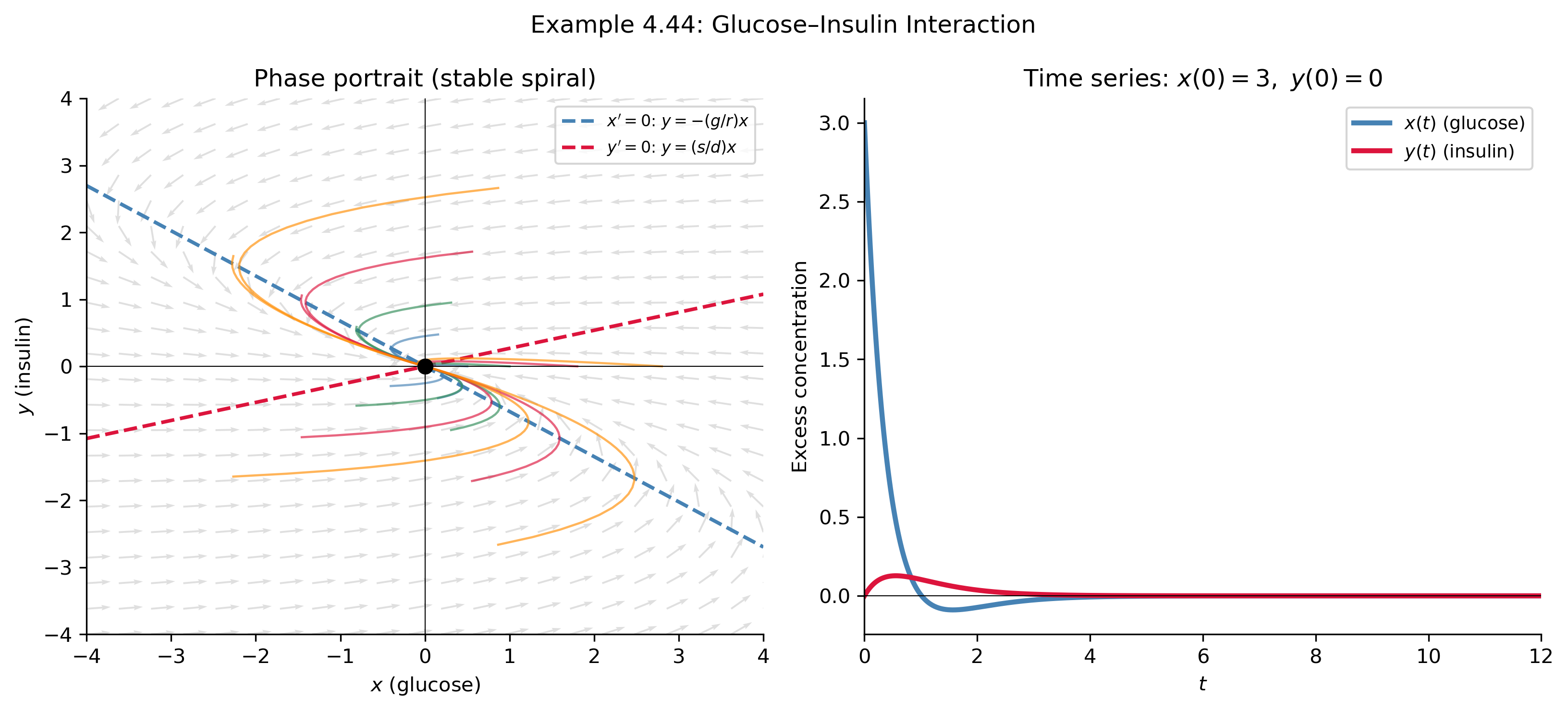
fig, axes = plt.subplots(1, 2, figsize=(11, 5))

lim = 4.0
x_g, y_g = np.meshgrid(np.linspace(-lim, lim, 22), np.linspace(-lim, lim, 22))
dx = A444[0,0]*x_g + A444[0,1]*y_g
dy = A444[1,0]*x_g + A444[1,1]*y_g
nrm = np.sqrt(dx**2 + dy**2 + 1e-10)
axes[0].quiver(x_g, y_g, dx/nrm, dy/nrm, alpha=0.25, color='gray', scale=28)

# Nullclines
x_nc = np.linspace(-lim, lim, 300)
axes[0].plot(x_nc, -(g_val/r_val)*x_nc, 'steelblue', ls='--', lw=1.8,
             label=r"$x'=0$: $y=-(g/r)x$")
axes[0].plot(x_nc, (s_val/d_val)*x_nc, 'crimson', ls='--', lw=1.8,
             label=r"$y'=0$: $y=(s/d)x$")

# Orbits
for r_frac, color in zip([0.5, 1.0, 1.8, 2.8],
                          ['steelblue', 'seagreen', 'crimson', 'darkorange']):
    for theta in np.linspace(0, 2*np.pi, 5, endpoint=False):
        x0 = [r_frac*np.cos(theta), r_frac*np.sin(theta)]
        sol = solve_ivp(lambda t, y: A444 @ y, (0, 8), x0,
                        dense_output=True, max_step=0.05)
        xy = sol.y; mask = np.all(np.abs(xy) < lim*1.4, axis=0)
        axes[0].plot(xy[0, mask], xy[1, mask], color=color, lw=1.1, alpha=0.65)

axes[0].axhline(0, color='k', lw=0.5); axes[0].axvline(0, color='k', lw=0.5)
axes[0].plot(0, 0, 'ko', markersize=7, zorder=5)
axes[0].set_xlim(-lim, lim); axes[0].set_ylim(-lim, lim)
axes[0].set_xlabel('$x$ (glucose)'); axes[0].set_ylabel('$y$ (insulin)')
axes[0].set_title('Phase portrait (stable spiral)')
axes[0].legend(fontsize=8)

# Time series starting at (3, 0)
t_plot = np.linspace(0, 12, 600)
sol_ts = solve_ivp(lambda t, y: A444 @ y, (0, 12), [3.0, 0.0],
                   dense_output=True, max_step=0.05)
axes[1].plot(t_plot, sol_ts.sol(t_plot)[0], color='steelblue', lw=2.5,
             label='$x(t)$ (glucose)')
axes[1].plot(t_plot, sol_ts.sol(t_plot)[1], color='crimson', lw=2.5,
             label='$y(t)$ (insulin)')
axes[1].axhline(0, color='k', lw=0.5)
axes[1].set_xlabel('$t$'); axes[1].set_ylabel('Excess concentration')
axes[1].set_title('Time series: $x(0)=3,\\ y(0)=0$')
axes[1].legend(fontsize=9)
axes[1].set_xlim(0, 12)

plt.suptitle("Example 4.44: Glucose–Insulin Interaction", fontsize=12)
plt.tight_layout()
plt.show()