Notes 4

Second-Order Linear Equations

Show the code
import numpy as np
import sympy as sym
import matplotlib as mpl
import matplotlib.pyplot as plt
from scipy.integrate import solve_ivp
from IPython.display import Math, display
mpl.rcParams['figure.dpi'] = 150
mpl.rcParams['axes.spines.top'] = False
mpl.rcParams['axes.spines.right'] = False

Goals

In this section we will cover the following topics:

  1. Introduce second-order linear ODEs with constant coefficients and their characteristic equation.

  2. Classify solutions according to the three cases for the characteristic roots (eigenvalues): distinct real, repeated real, and complex conjugate.

  3. Apply the method of undetermined coefficients to find particular solutions of inhomogeneous equations.

  4. Apply the method of variation of parameters as a general technique for finding particular solutions.

  5. Understand resonance — what happens when the forcing frequency matches the natural frequency.

Note

This material corresponds to Sections 2.2 and 2.3 of Logan (2015).


Second-Order Linear Equations: The Setup

A second-order linear ODE with constant coefficients has the form

\[ x'' + px' + qx = f(t), \tag{2} \]

where \(p\) and \(q\) are real constants and \(f(t)\) is a given function called the forcing term (or source term). When \(f(t) \equiv 0\) the equation is homogeneous; otherwise it is inhomogeneous.

This single equation encompasses an enormous range of physical models:

Application Equation
Simple harmonic oscillator \(x'' + \omega^2 x = 0\)
Damped oscillator \(x'' + 2\gamma x' + \omega^2 x = 0\)
Forced damped oscillator \(x'' + 2\gamma x' + \omega^2 x = F_0\cos(\Omega t)\)
RLC circuit \(LQ'' + RQ' + Q/C = E(t)\)
Euler–Bernoulli beam deflection (ODE form) \(EI\,y'' = M(x)\)

Structure of the general solution. By the Superposition Principle (discussed in detail in Topics 3), the general solution of the inhomogeneous equation (2) is: \[ x(t) = x_h(t) + x_p(t), \] where \(x_h\) is the general solution of the homogeneous equation \(x'' + px' + qx = 0\), and \(x_p\) is any particular solution of (2). We therefore study the homogeneous case first.


The Homogeneous Equation: Characteristic Equation

The Ansatz \(x = e^{\lambda t}\)

For the homogeneous equation \[ x'' + px' + qx = 0, \tag{H} \] we try the ansatz (educated guess) \(x(t) = e^{\lambda t}\), where \(\lambda\) is a constant to be determined. Substituting: \[ \lambda^2 e^{\lambda t} + p\lambda e^{\lambda t} + q e^{\lambda t} = 0. \] Since \(e^{\lambda t} \neq 0\) we can divide through by it, leaving the characteristic equation (also called the auxiliary equation):

\[ \boxed{\lambda^2 + p\lambda + q = 0.} \]

The values of \(\lambda\) satisfying this quadratic are called the eigenvalues of the equation. By the quadratic formula: \[ \lambda = \frac{-p \pm \sqrt{p^2 - 4q}}{2}. \]

The discriminant \(\Delta = p^2 - 4q\) determines which of three qualitatively different cases we are in.

NoteTerminology: Eigenvalues of a Differential Equation

Logan uses the term eigenvalue for the roots \(\lambda\) of the characteristic equation. This is appropriate: \(\lambda\) is precisely the value for which \(e^{\lambda t}\) is a solution of (H), and it plays the same conceptual role as an eigenvalue in linear algebra — it characterizes the modes of response of the system. We are not yet talking about matrix eigenvalues; that connection will emerge naturally when we convert higher-order ODEs to systems.


Case I — Two Distinct Real Eigenvalues (\(\Delta > 0\))

When \(\Delta = p^2 - 4q > 0\), there are two distinct real roots \(\lambda_1 \neq \lambda_2\). The functions \(e^{\lambda_1 t}\) and \(e^{\lambda_2 t}\) are both solutions of (H) and are linearly independent (since \(\lambda_1 \neq \lambda_2\)). By superposition, the general solution is: \[ \boxed{x(t) = C_1 e^{\lambda_1 t} + C_2 e^{\lambda_2 t}.} \]

NoteExample 1 — Distinct Real Eigenvalues

Solve \(x'' - 3x' + 2x = 0\).

Characteristic equation: \(\lambda^2 - 3\lambda + 2 = (\lambda-1)(\lambda-2) = 0\).

Eigenvalues: \(\lambda_1 = 1\), \(\lambda_2 = 2\).

General solution: \(x(t) = C_1 e^{t} + C_2 e^{2t}\).

Physical interpretation. When both eigenvalues are negative (\(\lambda_1 < \lambda_2 < 0\)), both exponentials decay and every solution tends to zero — the equilibrium is stable. When either eigenvalue is positive, the corresponding mode grows without bound — unstable. When eigenvalues have opposite signs, solutions behave like a saddle.


Case II — Repeated Real Eigenvalue (\(\Delta = 0\))

When \(\Delta = 0\), there is one repeated root \(\lambda_1 = \lambda_2 = -p/2\). The function \(e^{\lambda_1 t}\) is one solution, but we need a second, linearly independent solution. One can verify by direct substitution (the method of reduction of order) that \(t\,e^{\lambda_1 t}\) is also a solution. The general solution is: \[ \boxed{x(t) = \bigl(C_1 + C_2\,t\bigr)\,e^{\lambda_1 t}.} \]

NoteExample 2 — Repeated Eigenvalue

Solve \(x'' - 4x' + 4x = 0\).

Characteristic equation: \(\lambda^2 - 4\lambda + 4 = (\lambda - 2)^2 = 0\).

Eigenvalue: \(\lambda_1 = 2\) (repeated).

General solution: \(x(t) = (C_1 + C_2 t)\,e^{2t}\).

The repeated-eigenvalue case appears at the boundary between the oscillatory and non-oscillatory regimes and is called critical damping in mechanical and electrical applications.


Case III — Complex Conjugate Eigenvalues (\(\Delta < 0\))

When \(\Delta = p^2 - 4q < 0\), the roots are complex conjugates: \[ \lambda = \alpha \pm i\beta, \qquad \alpha = -\frac{p}{2}, \quad \beta = \frac{\sqrt{4q - p^2}}{2} > 0. \] The complex exponentials \(e^{(\alpha+i\beta)t}\) and \(e^{(\alpha-i\beta)t}\) are formally solutions, but we prefer real-valued solutions. Using Euler’s formula \(e^{i\beta t} = \cos(\beta t) + i\sin(\beta t)\) and taking real and imaginary parts, we obtain two real linearly independent solutions: \[ e^{\alpha t}\cos(\beta t) \quad\text{and}\quad e^{\alpha t}\sin(\beta t). \] The general solution is: \[ \boxed{x(t) = e^{\alpha t}\bigl(C_1\cos(\beta t) + C_2\sin(\beta t)\bigr).} \]

The solution oscillates at damped frequency \(\beta\) while its amplitude grows or decays like \(e^{\alpha t}\):

  • \(\alpha < 0\) (\(p > 0\)): underdamped — oscillations decay to zero.
  • \(\alpha = 0\) (\(p = 0\)): undamped — pure oscillation, amplitude constant.
  • \(\alpha > 0\) (\(p < 0\)): oscillations grow (unusual in passive physical systems).
NoteExample 3 — Complex Eigenvalues

Solve \(x'' + 2x' + 5x = 0\).

Characteristic equation: \(\lambda^2 + 2\lambda + 5 = 0\).

Eigenvalues: \(\lambda = \dfrac{-2 \pm \sqrt{4-20}}{2} = -1 \pm 2i\).

So \(\alpha = -1\), \(\beta = 2\).

General solution: \(x(t) = e^{-t}(C_1\cos(2t) + C_2\sin(2t))\).


Summary: The Three Cases

Show the code
t_plot = np.linspace(0, 5, 400)
fig, axes = plt.subplots(1, 3, figsize=(12, 4))

# ── Case I: Distinct real eigenvalues ───────────────────────
# x'' - 3x' + 2x = 0, lambda = 1, 2; x(0)=1, x'(0)=0
# x(0) = C1 + C2 = 1; x'(0) = C1 + 2*C2 = 0 => C2=-1, C1=2
C1, C2 = 2.0, -1.0
x_case1 = C1*np.exp(t_plot) + C2*np.exp(2*t_plot)
# Also show a stable case: x'' + 3x' + 2x = 0, lambda=-1,-2
# x(0)=1, x'(0)=0: C1+C2=1, -C1-2*C2=0 => C2=-1, C1=2... wait
# -C1-2*C2=0 => C1=-2C2; C1+C2=1 => -2C2+C2=1 => C2=-1, C1=2
C1s, C2s = 2.0, -1.0
x_stable = C1s*np.exp(-t_plot) + C2s*np.exp(-2*t_plot)
axes[0].plot(t_plot, x_case1, color='crimson', lw=2, label=r'$\lambda=1,2$ (unstable, $p=-3$)')
axes[0].plot(t_plot, x_stable, color='steelblue', lw=2, label=r'$\lambda=-1,-2$ (stable, $p=3$)')
axes[0].axhline(0, color='k', lw=0.5)
axes[0].set_xlabel('$t$'); axes[0].set_ylabel('$x(t)$')
axes[0].set_title('Case I: Distinct real $\lambda$')
axes[0].legend(fontsize=8); axes[0].set_ylim(-2, 5)

# ── Case II: Repeated eigenvalue ────────────────────────────
# x'' + 2*gamma*x' + gamma^2*x = 0 for various gamma
for gamma_val, color, lbl in zip([0.5, 1.0, 2.0],
                                  ['steelblue','darkorange','crimson'],
                                  [r'$\lambda=-0.5$ (rep.)',r'$\lambda=-1$ (rep.)',r'$\lambda=-2$ (rep.)']):
    # x(0)=1, x'(0)=0: C1=1, C2*lambda + C1*lambda*0 => diff and apply
    # x=(C1+C2t)e^(lambda*t); x(0)=C1=1; x'=(C2+lambda(C1+C2t))e^lambda*t
    # x'(0)=C2+lambda*C1=0 => C2=-lambda=gamma_val
    C1r, C2r = 1.0, gamma_val
    x_rep = (C1r + C2r*t_plot)*np.exp(-gamma_val*t_plot)
    axes[1].plot(t_plot, x_rep, color=color, lw=2, label=lbl)
axes[1].axhline(0, color='k', lw=0.5)
axes[1].set_xlabel('$t$'); axes[1].set_ylabel('$x(t)$')
axes[1].set_title('Case II: Repeated $\lambda$')
axes[1].legend(fontsize=8)

# ── Case III: Complex eigenvalues ───────────────────────────
# x'' + 2*gamma*x' + (gamma^2+beta^2)x=0; beta=2
beta = 2.0
for gamma_val, color, lbl in zip([0.0, 0.3, 0.8],
                                   ['steelblue','darkorange','crimson'],
                                   ['$\\gamma=0$ (undamped)','$\\gamma=0.3$ (underdamped)','$\\gamma=0.8$ (underdamped)']):
    # x(0)=1, x'(0)=0: C1=1, alpha*C1 + beta*C2=0 => C2=gamma/beta
    C1c = 1.0
    C2c = gamma_val / beta
    x_complex = np.exp(-gamma_val*t_plot)*(C1c*np.cos(beta*t_plot) + C2c*np.sin(beta*t_plot))
    axes[2].plot(t_plot, x_complex, color=color, lw=2, label=lbl)
# Envelope
axes[2].plot(t_plot,  np.exp(-0.3*t_plot), color='darkorange', lw=1, ls=':', alpha=0.8)
axes[2].plot(t_plot, -np.exp(-0.3*t_plot), color='darkorange', lw=1, ls=':', alpha=0.8)
axes[2].axhline(0, color='k', lw=0.5)
axes[2].set_xlabel('$t$'); axes[2].set_ylabel('$x(t)$')
axes[2].set_title('Case III: Complex $\\lambda = \\alpha\\pm i\\beta$')
axes[2].legend(fontsize=8)

plt.suptitle('Three Cases of the Characteristic Equation', fontsize=12)
plt.tight_layout()
plt.show()
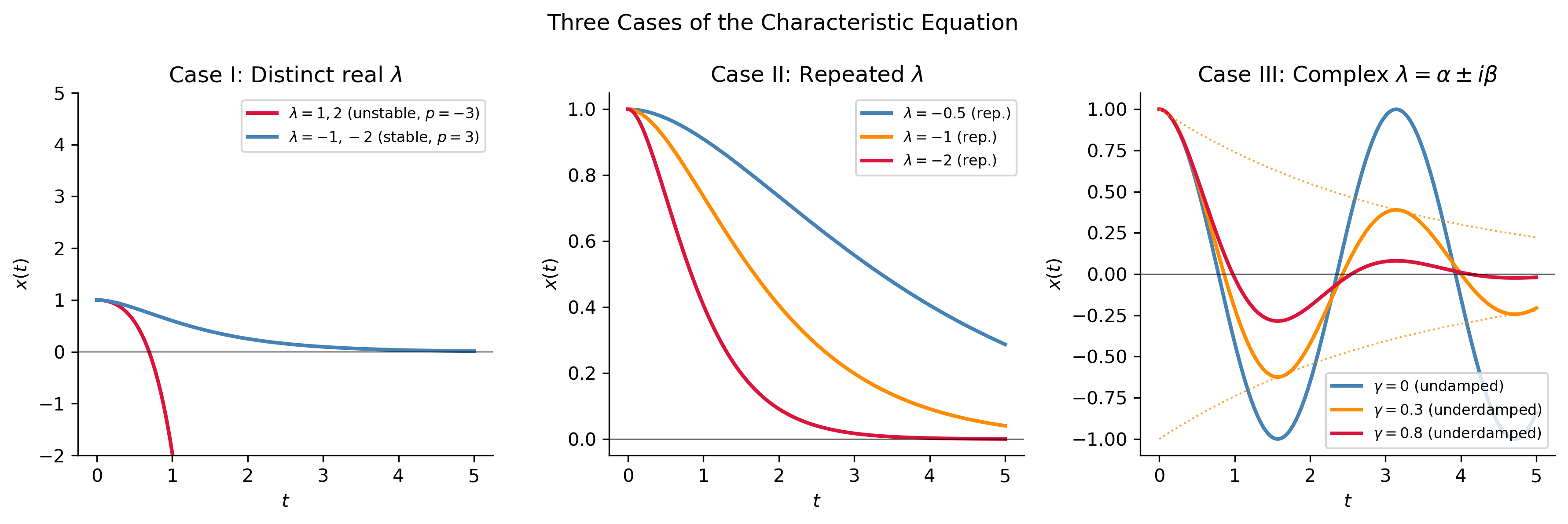
Figure 1: Representative solutions for each of the three cases of the characteristic equation. All equations have the form \(x''+px'+qx=0\) with initial conditions \(x(0)=1\), \(x'(0)=0\). Left: distinct real eigenvalues (exponential behavior). Middle: repeated eigenvalue (critical damping). Right: complex eigenvalues (oscillatory decay — underdamped).

The Damped Harmonic Oscillator

The equation \[ x'' + 2\gamma x' + \omega_0^2\,x = 0 \] governs a mass on a spring with damping coefficient \(2\gamma > 0\) and natural frequency \(\omega_0\). The characteristic equation is \(\lambda^2 + 2\gamma\lambda + \omega_0^2 = 0\), giving \(\lambda = -\gamma \pm \sqrt{\gamma^2 - \omega_0^2}\).

The three cases are:

Regime Condition Eigenvalues Solution behavior
Overdamped \(\gamma > \omega_0\) Two distinct negative reals Exponential decay, no oscillation
Critically damped \(\gamma = \omega_0\) Repeated \(\lambda = -\gamma\) Fastest non-oscillatory decay
Underdamped \(\gamma < \omega_0\) \(-\gamma \pm i\omega_d\) Oscillatory decay at \(\omega_d = \sqrt{\omega_0^2-\gamma^2}\)

where \(\omega_d\) is the damped natural frequency.

Show the code
omega0 = 1.0
t_plot = np.linspace(0, 12, 600)

fig, axes = plt.subplots(1, 2, figsize=(11, 4.5))

# ── All three regimes ───────────────────────────────────────
def dho(t, y, gamma, omega0):
    return [y[1], -2*gamma*y[1] - omega0**2*y[0]]

params = [(0.1, 'steelblue',   'Underdamped $\\gamma=0.1$'),
          (1.0, 'darkorange',  'Critically damped $\\gamma=1.0$'),
          (2.0, 'crimson',     'Overdamped $\\gamma=2.0$')]

for gamma, color, lbl in params:
    sol = solve_ivp(dho, (0,12), [1.0, 0.0], args=(gamma, omega0),
                    t_eval=t_plot, max_step=0.02)
    axes[0].plot(sol.t, sol.y[0], color=color, lw=2, label=lbl)

axes[0].axhline(0, color='k', lw=0.5)
axes[0].set_xlabel('$t$'); axes[0].set_ylabel('$x(t)$')
axes[0].set_title(r'Three damping regimes ($\omega_0=1$, $x(0)=1$, $x\'(0)=0$)')
axes[0].legend(fontsize=8.5)

# ── Phase portrait ──────────────────────────────────────────
for gamma, color, lbl in params:
    sol = solve_ivp(dho, (0,12), [1.0, 0.0], args=(gamma, omega0),
                    t_eval=t_plot, max_step=0.02)
    axes[1].plot(sol.y[0], sol.y[1], color=color, lw=2, label=lbl)
axes[1].plot(1, 0, 'ko', markersize=7, label='IC $(1,0)$', zorder=5)
axes[1].plot(0, 0, 'k*', markersize=10, label='Origin (equilibrium)', zorder=5)
axes[1].set_xlabel('$x$'); axes[1].set_ylabel("$x'$")
axes[1].set_title('Phase portrait')
axes[1].legend(fontsize=8)
axes[1].set_aspect('equal')

plt.tight_layout()
plt.show()
Figure 2: Damped harmonic oscillator \(x''+2\gamma x'+x=0\) (\(\omega_0=1\)) from initial conditions \(x(0)=1\), \(x'(0)=0\). The three damping regimes show qualitatively different behavior. In the underdamped case the dotted curve shows the decaying amplitude envelope \(\pm e^{-\gamma t}\).

Solving IVPs for Second-Order Equations

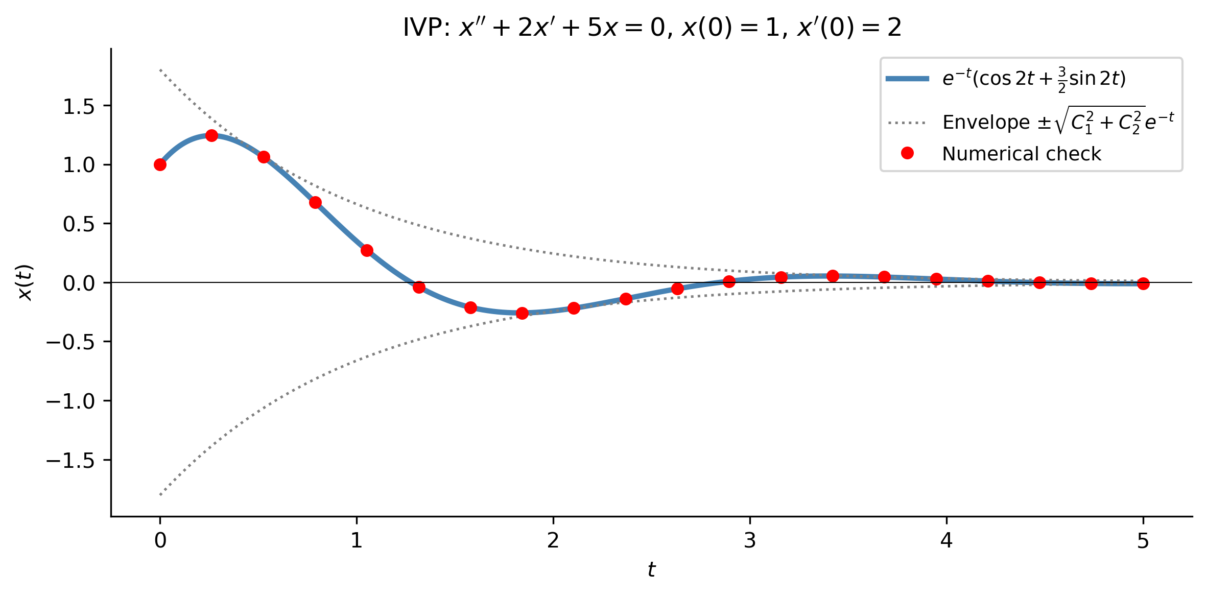
Example 4. Solve the IVP: \(x'' + 2x' + 5x = 0\), \(x(0)=1\), \(x'(0)=2\).

Step 1 — Characteristic equation: \(\lambda^2 + 2\lambda + 5 = 0 \Rightarrow \lambda = -1 \pm 2i\).

Step 2 — General solution: \(x(t) = e^{-t}(C_1\cos 2t + C_2\sin 2t)\).

Step 3 — Apply ICs. At \(t=0\): \[x(0) = C_1 = 1.\] Differentiating: \(x'(t) = -e^{-t}(C_1\cos 2t + C_2\sin 2t) + e^{-t}(-2C_1\sin 2t + 2C_2\cos 2t)\). \[x'(0) = -C_1 + 2C_2 = 2 \;\Rightarrow\; C_2 = \tfrac{3}{2}.\]

Solution: \(\displaystyle x(t) = e^{-t}\!\left(\cos 2t + \tfrac{3}{2}\sin 2t\right)\).

Show the code
# Verify with SymPy
t_sym = sym.Symbol('t')
x_sym = sym.Function('x')
ode_ex4 = sym.Eq(x_sym(t_sym).diff(t_sym,2) + 2*x_sym(t_sym).diff(t_sym) + 5*x_sym(t_sym), 0)
sol_ex4 = sym.dsolve(ode_ex4, x_sym(t_sym),
                     ics={x_sym(0): 1, x_sym(t_sym).diff(t_sym).subs(t_sym,0): 2})
print("IVP solution:")
display(Math(sym.latex(sol_ex4)))
IVP solution:

\(\displaystyle x{\left(t \right)} = \left(\frac{3 \sin{\left(2 t \right)}}{2} + \cos{\left(2 t \right)}\right) e^{- t}\)

Show the code
t_plot = np.linspace(0, 5, 400)
x_sol = np.exp(-t_plot)*(np.cos(2*t_plot) + 1.5*np.sin(2*t_plot))
envelope = np.sqrt(1 + 1.5**2) * np.exp(-t_plot)   # amplitude = sqrt(C1^2+C2^2)

def ode_num(t, y): return [y[1], -2*y[1] - 5*y[0]]
sol_num = solve_ivp(ode_num, (0,5), [1.0, 2.0], dense_output=True, max_step=0.02)

fig, ax = plt.subplots(figsize=(8, 4))
ax.plot(t_plot, x_sol, color='steelblue', lw=2.5, label=r'$e^{-t}(\cos 2t+\frac{3}{2}\sin 2t)$')
ax.plot(t_plot,  envelope, color='gray', lw=1.2, ls=':', label='Envelope $\\pm\\sqrt{C_1^2+C_2^2}e^{-t}$')
ax.plot(t_plot, -envelope, color='gray', lw=1.2, ls=':')
t_dots = np.linspace(0, 5, 20)
ax.plot(t_dots, sol_num.sol(t_dots)[0], 'ro', markersize=5, label='Numerical check')
ax.axhline(0, color='k', lw=0.5)
ax.set_xlabel('$t$'); ax.set_ylabel('$x(t)$')
ax.set_title(r"IVP: $x''+2x'+5x=0$, $x(0)=1$, $x'(0)=2$")
ax.legend(fontsize=9)
plt.tight_layout()
plt.show()
Figure 3: Solution to the IVP \(x''+2x'+5x=0\), \(x(0)=1\), \(x'(0)=2\) (Example 4). The solution oscillates with frequency \(\beta=2\) while the amplitude decays like \(e^{-t}\) (dotted envelope). Red dots are a numerical check via solve_ivp.

Using SymPy for Second-Order Constant-Coefficient ODEs

Show the code
t_sym = sym.Symbol('t')
x_sym = sym.Function('x')

cases = {
    r"x'' - 3x' + 2x = 0 \;\;(\Delta>0)":
        x_sym(t_sym).diff(t_sym,2) - 3*x_sym(t_sym).diff(t_sym) + 2*x_sym(t_sym),
    r"x'' - 4x' + 4x = 0 \;\;(\Delta=0)":
        x_sym(t_sym).diff(t_sym,2) - 4*x_sym(t_sym).diff(t_sym) + 4*x_sym(t_sym),
    r"x'' + 2x' + 5x = 0 \;\;(\Delta<0)":
        x_sym(t_sym).diff(t_sym,2) + 2*x_sym(t_sym).diff(t_sym) + 5*x_sym(t_sym),
}

for label, expr in cases.items():
    ode = sym.Eq(expr, 0)
    sol = sym.dsolve(ode, x_sym(t_sym))
    print(f"ODE: ${label}$")
    display(Math(r"x(t) = " + sym.latex(sol.rhs)))
    print()
ODE: $x'' - 3x' + 2x = 0 \;\;(\Delta>0)$

\(\displaystyle x(t) = \left(C_{1} + C_{2} e^{t}\right) e^{t}\)


ODE: $x'' - 4x' + 4x = 0 \;\;(\Delta=0)$

\(\displaystyle x(t) = \left(C_{1} + C_{2} t\right) e^{2 t}\)


ODE: $x'' + 2x' + 5x = 0 \;\;(\Delta<0)$

\(\displaystyle x(t) = \left(C_{1} \sin{\left(2 t \right)} + C_{2} \cos{\left(2 t \right)}\right) e^{- t}\)


Nonhomogeneous Equations

We now turn to the inhomogeneous equation \[ x'' + px' + qx = f(t). \tag{NH} \] The general solution is \(x(t) = x_h(t) + x_p(t)\), where \(x_h\) is the general solution of the homogeneous equation and \(x_p\) is any particular solution. We study two methods for finding \(x_p\).


Method of Undetermined Coefficients

The method of undetermined coefficients works when \(f(t)\) belongs to the family of functions closed under differentiation — polynomials, exponentials, sines, cosines, and their products. The idea is to guess the form of \(x_p\) based on \(f(t)\), leaving coefficients to be determined by substitution.

ImportantGuessing Table for Undetermined Coefficients
Forcing \(f(t)\) Guess for \(x_p\)
\(P_n(t)\) (polynomial degree \(n\)) \(A_n t^n + A_{n-1}t^{n-1} + \cdots + A_0\)
\(e^{at}\) \(Ae^{at}\)
\(\cos(\omega t)\) or \(\sin(\omega t)\) \(A\cos(\omega t) + B\sin(\omega t)\)
\(e^{at}\cos(\omega t)\) or \(e^{at}\sin(\omega t)\) \(e^{at}(A\cos(\omega t) + B\sin(\omega t))\)
\(P_n(t)e^{at}\) \((A_n t^n+\cdots+A_0)e^{at}\)

Modification rule. If the guessed form \(x_p\) overlaps with a term in \(x_h\) (i.e., it would be annihilated by the homogeneous operator), multiply the guess by \(t\) (or \(t^2\) if there is a repeated overlap).


Example 5 — Exponential Forcing

Solve \(x'' + 2x' + 5x = 3e^t\).

Step 1 — Homogeneous solution (from Example 3): \(x_h = e^{-t}(C_1\cos 2t + C_2\sin 2t)\).

Step 2 — Guess \(x_p = Ae^t\) (since \(e^t\) is not in \(x_h\)).

Step 3 — Substitute: \[A e^t + 2Ae^t + 5Ae^t = 8Ae^t = 3e^t \;\Rightarrow\; A = \tfrac{3}{8}.\]

General solution: \[x(t) = e^{-t}(C_1\cos 2t + C_2\sin 2t) + \tfrac{3}{8}e^t.\]


Example 6 — Polynomial Forcing

Solve \(x'' + x' - 2x = t^2\).

Step 1 — Characteristic equation: \(\lambda^2 + \lambda - 2 = (\lambda-1)(\lambda+2) = 0 \Rightarrow \lambda = 1, -2\).

Homogeneous solution: \(x_h = C_1 e^t + C_2 e^{-2t}\).

Step 2 — Guess \(x_p = At^2 + Bt + C\) (degree-2 polynomial).

Step 3 — Substitute: \[2A + (2At + B) - 2(At^2 + Bt + C) = -2At^2 + (2A-2B)t + (2A+B-2C) = t^2.\]

Equating coefficients: \[-2A = 1 \;\Rightarrow\; A = -\tfrac{1}{2}; \quad 2A - 2B = 0 \;\Rightarrow\; B = -\tfrac{1}{2}; \quad 2A + B - 2C = 0 \;\Rightarrow\; C = -\tfrac{3}{4}.\]

General solution: \[x(t) = C_1 e^t + C_2 e^{-2t} - \tfrac{1}{2}t^2 - \tfrac{1}{2}t - \tfrac{3}{4}.\]

Show the code
t_sym = sym.Symbol('t')
x_sym = sym.Function('x')

# Example 5
ode5 = sym.Eq(x_sym(t_sym).diff(t_sym,2) + 2*x_sym(t_sym).diff(t_sym) + 5*x_sym(t_sym),
              3*sym.exp(t_sym))
sol5 = sym.dsolve(ode5, x_sym(t_sym))
print("Example 5 (exponential forcing):")
display(Math(r"x(t) = " + sym.latex(sol5.rhs)))
print()

# Example 6
ode6 = sym.Eq(x_sym(t_sym).diff(t_sym,2) + x_sym(t_sym).diff(t_sym) - 2*x_sym(t_sym),
              t_sym**2)
sol6 = sym.dsolve(ode6, x_sym(t_sym))
print("Example 6 (polynomial forcing):")
display(Math(r"x(t) = " + sym.latex(sol6.rhs)))
Example 5 (exponential forcing):

\(\displaystyle x(t) = \left(C_{1} \sin{\left(2 t \right)} + C_{2} \cos{\left(2 t \right)}\right) e^{- t} + \frac{3 e^{t}}{8}\)


Example 6 (polynomial forcing):

\(\displaystyle x(t) = C_{1} e^{- 2 t} + C_{2} e^{t} - \frac{t^{2}}{2} - \frac{t}{2} - \frac{3}{4}\)


Resonance

Resonance occurs when the frequency of the forcing matches the natural frequency of the homogeneous equation. This is when the modification rule is essential.

NoteExample 7 — Non-Resonant Forcing

Solve \(x'' + 4x = \cos(t)\).

Natural frequency: \(\omega_0 = 2\) (from \(x'' + 4x = 0\)).

Guess \(x_p = A\cos t + B\sin t\) (frequency \(\omega=1 \neq 2\), no overlap with \(x_h\)).

Substitute: \((-A\cos t - B\sin t) + 4(A\cos t + B\sin t) = 3A\cos t + 3B\sin t = \cos t\).

So \(A = 1/3\), \(B = 0\), giving \(x_p = \dfrac{\cos t}{3}\).

General solution: \(x(t) = C_1\cos(2t) + C_2\sin(2t) + \dfrac{\cos t}{3}\).

ImportantExample 8 — Resonance

Solve \(x'' + 4x = \cos(2t)\).

Natural frequency: \(\omega_0 = 2\) — the forcing frequency equals the natural frequency.

Initial guess \(A\cos(2t) + B\sin(2t)\) overlaps with \(x_h\) — use the modification rule and multiply by \(t\): \[x_p = t\bigl(A\cos(2t) + B\sin(2t)\bigr).\]

Substitute (after computing \(x_p''\) carefully): \[x_p'' + 4x_p = -4A\sin(2t) + 4B\cos(2t) = \cos(2t).\]

So \(A = 0\), \(B = 1/4\), giving \(\displaystyle x_p = \frac{t\sin(2t)}{4}\).

General solution: \(x(t) = C_1\cos(2t) + C_2\sin(2t) + \dfrac{t\sin(2t)}{4}\).

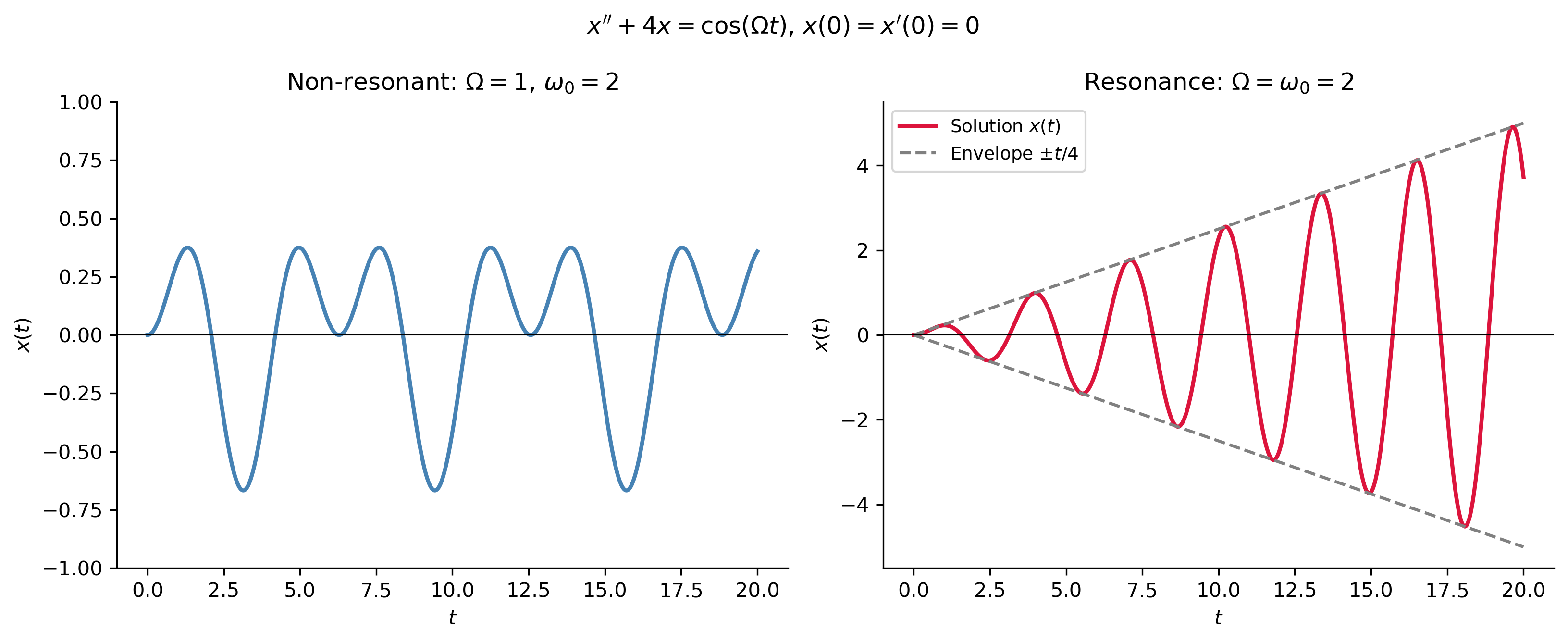
The particular solution \(x_p = t\sin(2t)/4\) grows linearly in amplitude — this is the signature of resonance. With zero initial conditions, the full solution oscillates with an amplitude that grows without bound.

Show the code
t_plot = np.linspace(0, 20, 1000)

def forced_osc(t, y, Omega):
    return [y[1], -4*y[0] + np.cos(Omega*t)]

fig, axes = plt.subplots(1, 2, figsize=(11, 4.5))

# Non-resonant
sol_nr = solve_ivp(forced_osc, (0,20), [0,0], args=(1.0,), t_eval=t_plot, max_step=0.02)
axes[0].plot(sol_nr.t, sol_nr.y[0], color='steelblue', lw=2)
axes[0].axhline(0, color='k', lw=0.5)
axes[0].set_xlabel('$t$'); axes[0].set_ylabel('$x(t)$')
axes[0].set_title(r"Non-resonant: $\Omega=1$, $\omega_0=2$")
axes[0].set_ylim(-1, 1)

# Resonant
sol_r = solve_ivp(forced_osc, (0,20), [0,0], args=(2.0,), t_eval=t_plot, max_step=0.02)
axes[1].plot(sol_r.t, sol_r.y[0], color='crimson', lw=2, label='Solution $x(t)$')
axes[1].plot(t_plot,  t_plot/4, color='gray', lw=1.5, ls='--', label='Envelope $\\pm t/4$')
axes[1].plot(t_plot, -t_plot/4, color='gray', lw=1.5, ls='--')
axes[1].axhline(0, color='k', lw=0.5)
axes[1].set_xlabel('$t$'); axes[1].set_ylabel('$x(t)$')
axes[1].set_title(r"Resonance: $\Omega=\omega_0=2$")
axes[1].legend(fontsize=9)

plt.suptitle(r"$x'' + 4x = \cos(\Omega t)$, $x(0)=x'(0)=0$", fontsize=12)
plt.tight_layout()
plt.show()
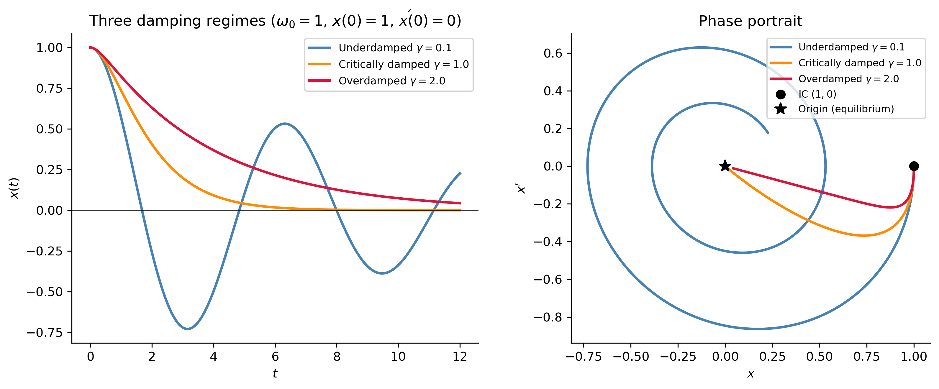
Figure 4: Resonance vs. non-resonance for \(x''+4x=\cos(\Omega t)\) with \(x(0)=x'(0)=0\). Left: non-resonant (\(\Omega=1\)) — bounded steady-state oscillation. Right: resonant (\(\Omega=2=\omega_0\)) — amplitude grows linearly without bound. The dashed line shows the linear growth envelope \(\pm t/4\).
TipResonance in Practice

Resonance is not merely a mathematical curiosity. It has caused real engineering disasters, including the Tacoma Narrows Bridge collapse (1940), where aerodynamic forcing matched the bridge’s natural torsional frequency. It is also deliberately exploited in technology: MRI scanners use radio-frequency pulses tuned to the resonant frequency of nuclear spins; musical instruments are designed so their resonant frequencies match desired notes.


Variation of Parameters

The method of undetermined coefficients requires \(f(t)\) to have a specific form. Variation of parameters (developed by Lagrange) works for any continuous \(f(t)\).

Setup. Let \(x_1(t)\) and \(x_2(t)\) be two linearly independent solutions of the homogeneous equation, forming the general homogeneous solution \(x_h = C_1 x_1 + C_2 x_2\). We seek a particular solution of the form \[ x_p(t) = u_1(t)\,x_1(t) + u_2(t)\,x_2(t), \] where \(u_1(t)\) and \(u_2(t)\) are now functions to be determined (hence “variation of parameters” — the parameters \(C_1, C_2\) are allowed to vary).

Derivation. Imposing the constraint \(u_1'x_1 + u_2'x_2 = 0\) (which eliminates second derivatives of \(u_1\), \(u_2\) from the substitution) and substituting into (NH) yields the system: \[ u_1'x_1 + u_2'x_2 = 0, \qquad u_1'x_1' + u_2'x_2' = f(t). \] This linear system for \(u_1'\) and \(u_2'\) has coefficient determinant equal to the Wronskian: \[ W(x_1, x_2) = x_1 x_2' - x_2 x_1', \] which is nonzero since \(x_1\), \(x_2\) are linearly independent. Solving by Cramer’s rule: \[ u_1' = -\frac{x_2\,f}{W}, \qquad u_2' = \frac{x_1\,f}{W}. \]

ImportantVariation of Parameters Formula

\[ x_p(t) = -x_1(t)\int\frac{x_2(t)\,f(t)}{W(t)}\,dt + x_2(t)\int\frac{x_1(t)\,f(t)}{W(t)}\,dt. \]


Example 9 — Variation of Parameters

Solve \(x'' + 4x = \sec(2t)\).

This forcing function is not in the guessing table for undetermined coefficients, so we use variation of parameters.

Homogeneous solutions: \(x_1 = \cos(2t)\), \(x_2 = \sin(2t)\).

Wronskian: \[W = x_1 x_2' - x_2 x_1' = \cos(2t)\cdot 2\cos(2t) - \sin(2t)\cdot(-2\sin(2t)) = 2.\]

Compute \(u_1'\) and \(u_2'\): \[u_1' = -\frac{\sin(2t)\cdot\sec(2t)}{2} = -\frac{\tan(2t)}{2}, \qquad u_2' = \frac{\cos(2t)\cdot\sec(2t)}{2} = \frac{1}{2}.\]

Integrate: \[u_1 = \frac{\ln|\cos(2t)|}{4}, \qquad u_2 = \frac{t}{2}.\]

Particular solution: \[x_p = \frac{\cos(2t)\ln|\cos(2t)|}{4} + \frac{t\sin(2t)}{2}.\]

General solution: \[x(t) = C_1\cos(2t) + C_2\sin(2t) + \frac{\cos(2t)\ln|\cos(2t)|}{4} + \frac{t\sin(2t)}{2}.\]

Show the code
# Verify with SymPy
t_sym = sym.Symbol('t')
x_sym = sym.Function('x')
ode9 = sym.Eq(x_sym(t_sym).diff(t_sym,2) + 4*x_sym(t_sym), sym.sec(2*t_sym))
sol9 = sym.dsolve(ode9, x_sym(t_sym))
print("Example 9 (variation of parameters):")
display(Math(r"x(t) = " + sym.latex(sol9.rhs)))
Example 9 (variation of parameters):

\(\displaystyle x(t) = \left(C_{1} + \frac{t}{2}\right) \sin{\left(2 t \right)} + \left(C_{2} + \frac{\log{\left(\cos{\left(2 t \right)} \right)}}{4}\right) \cos{\left(2 t \right)}\)

Show the code
# Solution with ICs x(0)=1, x'(0)=0 on a restricted domain
# xp(0) = (1/4)*ln(1) + 0 = 0; xp'(0) = -sin(0)*ln(cos(0))/4*2 + ...
# Just plot numerically to avoid the singularity
def ode9_num(t, y):
    if abs(np.cos(2*t)) < 1e-6:
        return [y[1], 0.0]
    return [y[1], -4*y[0] + 1/np.cos(2*t)]

t_span = (0, np.pi/4 - 0.05)
t_eval = np.linspace(0, np.pi/4 - 0.05, 400)
sol9_num = solve_ivp(ode9_num, t_span, [1.0, 0.0], t_eval=t_eval, max_step=0.005)

fig, ax = plt.subplots(figsize=(8, 4))
ax.plot(sol9_num.t, sol9_num.y[0], color='steelblue', lw=2.5,
        label=r'$x(t)$ on $[0, \pi/4)$')
ax.axvline(np.pi/4, color='crimson', ls='--', lw=1.5,
           label=r'Singularity at $t=\pi/4$')
ax.set_xlabel('$t$'); ax.set_ylabel('$x(t)$')
ax.set_title(r"$x''+4x=\sec(2t)$ via variation of parameters")
ax.legend(fontsize=9)
plt.tight_layout()
plt.show()
Figure 5: Solution to \(x''+4x=\sec(2t)\) via variation of parameters with \(x(0)=1\), \(x'(0)=0\) (particular solution plus homogeneous solution to match ICs). The forcing \(\sec(2t)\) becomes singular at \(t=\pi/4\approx 0.785\), limiting the interval of existence.

Comparing the Two Methods

Feature Undetermined Coefficients Variation of Parameters
Applicability \(f(t)\) must be a polynomial, exponential, or trig function Any continuous \(f(t)\)
Difficulty Simple algebra Requires integration (may be hard)
Resonance Handled by modification rule Handles automatically
When to use First choice for standard forcing When undetermined coefficients fails

Summary

Concept Key Formula
Characteristic equation \(\lambda^2 + p\lambda + q = 0\)
Case I (\(\Delta>0\)) \(x = C_1 e^{\lambda_1 t} + C_2 e^{\lambda_2 t}\)
Case II (\(\Delta=0\)) \(x = (C_1 + C_2 t)e^{\lambda t}\)
Case III (\(\Delta<0\)) \(x = e^{\alpha t}(C_1\cos\beta t + C_2\sin\beta t)\)
General solution \(x = x_h + x_p\)
Undetermined coefficients Guess form of \(x_p\) from \(f(t)\); modify if overlap with \(x_h\)
Variation of parameters \(u_1'x_1+u_2'x_2=0\), \(u_1'x_1'+u_2'x_2'=f\); integrate
Resonance Forcing at \(\omega_0\) → amplitude grows like \(t\)
TipLooking Ahead

The machinery developed here — characteristic equations, eigenvalues, and the superposition principle — extends directly to systems of first-order ODEs. A second-order ODE \(x''+px'+qx=0\) is equivalent to the 2D system \(\mathbf{y}' = A\mathbf{y}\) with \(A = \bigl[\begin{smallmatrix} 0 & 1 \\ -q & -p \end{smallmatrix}\bigr]\). The eigenvalues of \(A\) (in the matrix sense) are exactly the roots \(\lambda\) of \(\lambda^2+p\lambda+q=0\) — the two notions of eigenvalue coincide. This connection is developed in Chapter 3 of Logan (2015).


These notes are also viewable as a slide deck presentation: Open slides in full screen

Note

Next: Variation of parameters for second-order linear equations — Logan §2.4.


Relevant Videos

How to solve constant-coefficient second-order ODEs:

The different root scenarios for constant-coefficient second-order ODEs:

Two Examples of Undetermined Coefficients:

References

Logan, J David. 2015. A First Course in Differential Equations Third Edition.
Show the code
import sys
print("Python version:", sys.version)
print('\n'.join(f'{m.__name__}=={m.__version__}' for m in globals().values() if getattr(m, '__version__', None)))
Python version: 3.14.4 | packaged by conda-forge | (main, Apr  8 2026, 02:33:53) [Clang 20.1.8 ]
numpy==2.4.3
sympy==1.14.0
matplotlib==3.10.8