Notes 3

One-Dimensional Dynamical Systems

Show the code
import numpy as np
import sympy as sym
import matplotlib as mpl
import matplotlib.pyplot as plt
from scipy.integrate import solve_ivp
from IPython.display import Math, display
mpl.rcParams['figure.dpi'] = 150
mpl.rcParams['axes.spines.top'] = False
mpl.rcParams['axes.spines.right'] = False

Goals

In this section, we will cover the following topics:

  1. Introduce autonomous first-order ODEs \(x' = f(x)\) as one-dimensional dynamical systems.

  2. Define equilibrium solutions and analyze their stability using the phase line.

  3. Use linearization — evaluating \(f'(x^*)\) at an equilibrium — to determine stability analytically.

  4. Study bifurcations: qualitative changes in the equilibrium structure as a parameter varies, and how to construct bifurcation diagrams.

Note

This material corresponds to Section 1.5 of Logan (2015).


Autonomous Equations and Dynamical Systems

The Setup

An autonomous ODE is one in which the independent variable \(t\) does not appear explicitly on the right-hand side: \[ x' = f(x). \] The word autonomous means self-governing: the rate of change of \(x\) depends only on the current state \(x\), not on the time at which that state is reached. Contrast this with a non-autonomous equation such as \(x' = tx\), where the same state \(x\) at different times produces different rates of change.

A first-order autonomous ODE defines a one-dimensional dynamical system: a rule that tells us how a single quantity \(x\) — a population, a temperature, a voltage — evolves over time.

Key observation. For an autonomous ODE, the slope field has a particularly simple structure: the slope \(f(x)\) is constant along every horizontal line \(x = c\). This means the qualitative behavior of all solutions can be read directly from the graph of \(f\) as a function of \(x\) alone, without solving the ODE.


Equilibrium Solutions

ImportantDefinition: Equilibrium Solution

An equilibrium solution (also called a steady state or fixed point) of \(x' = f(x)\) is a constant solution \(x(t) \equiv x^*\) for all \(t\). It satisfies \[ f(x^*) = 0. \] Geometrically, equilibria are the zeros of \(f\) — the values of \(x\) where the slope field is horizontal.

Because an equilibrium solution is constant, it corresponds to a horizontal line in the \(tx\)-plane, and to a point on the \(x\)-axis (the phase line, introduced below).


The Phase Line

Since \(f\) depends only on \(x\), we can capture the entire qualitative behavior of the dynamical system in a single one-dimensional picture called the phase line (or phase portrait for 1D systems).

ImportantConstructing the Phase Line
  1. Find all equilibria by solving \(f(x^*) = 0\). Mark them on the \(x\)-axis.
  2. On each interval between equilibria, determine the sign of \(f(x)\):
    • \(f(x) > 0\): solutions are increasing (\(x\) moves right \(\rightarrow\)).
    • \(f(x) < 0\): solutions are decreasing (\(x\) moves left \(\leftarrow\)).
  3. Draw arrows on the \(x\)-axis pointing in the direction of flow.

The phase line immediately reveals the long-time behavior of every solution.


Stability of Equilibria

ImportantDefinitions: Stability

An equilibrium \(x^*\) is:

  • Stable (or asymptotically stable): if solutions starting near \(x^*\) converge to \(x^*\) as \(t \to \infty\). On the phase line, arrows on both sides point toward \(x^*\).

  • Unstable: if solutions starting near \(x^*\) move away from \(x^*\). On the phase line, arrows on both sides point away from \(x^*\).

  • Semi-stable: if arrows point toward \(x^*\) on one side and away on the other.


Example 1 — The Logistic Equation

\[ x' = rx\!\left(1 - \frac{x}{K}\right), \quad r > 0,\; K > 0. \]

Equilibria: \(f(x) = rx(1-x/K) = 0 \Rightarrow x^* = 0\) and \(x^* = K\).

Sign analysis:

  • \(x < 0\): \(f < 0\) (decreasing)
  • \(0 < x < K\): \(f > 0\) (increasing)
  • \(x > K\): \(f < 0\) (decreasing)

So \(x^* = 0\) is unstable and \(x^* = K\) is stable.

Show the code
r_val, K_val = 1.0, 4.0
f_log = lambda x: r_val * x * (1 - x / K_val)
x_arr = np.linspace(-0.5, 6.5, 400)
f_arr = f_log(x_arr)

fig = plt.figure(figsize=(11, 5))
gs  = fig.add_gridspec(2, 2, width_ratios=[1.8, 1], hspace=0.5, wspace=0.35)
ax_f  = fig.add_subplot(gs[0, 0])
ax_pl = fig.add_subplot(gs[1, 0])
ax_t  = fig.add_subplot(gs[:, 1])

# ── f(x) graph ──────────────────────────────────────────────
ax_f.plot(x_arr, f_arr, color='steelblue', lw=2.5)
ax_f.axhline(0, color='k', lw=0.8)
ax_f.fill_between(x_arr, 0, f_arr, where=(f_arr > 0),
                  alpha=0.15, color='seagreen', label='$f>0$ (increasing)')
ax_f.fill_between(x_arr, 0, f_arr, where=(f_arr < 0),
                  alpha=0.15, color='crimson',  label='$f<0$ (decreasing)')
ax_f.plot([0, K_val], [0, 0], 'ko', markersize=8, zorder=5)
ax_f.set_xlabel('$x$'); ax_f.set_ylabel("$f(x)$")
ax_f.set_title(r"$f(x)=x(1-x/4)$"); ax_f.legend(fontsize=8)
ax_f.set_xlim(-0.5, 6.5)

# ── Phase line ───────────────────────────────────────────────
ax_pl.axhline(0, color='k', lw=1.2)
ax_pl.plot(0,     0, 'o', markersize=12, color='crimson',  zorder=5)
ax_pl.plot(K_val, 0, 'o', markersize=12, color='seagreen', zorder=5)
ax_pl.annotate('', xy=(-0.3, 0), xytext=(0.3, 0),
               arrowprops=dict(arrowstyle='<-', color='crimson', lw=2))
for xm in [1.5, 2.5]:
    ax_pl.annotate('', xy=(xm+0.5, 0), xytext=(xm-0.5, 0),
                   arrowprops=dict(arrowstyle='->', color='seagreen', lw=2))
for xm in [5.0, 5.8]:
    ax_pl.annotate('', xy=(xm-0.5, 0), xytext=(xm+0.5, 0),
                   arrowprops=dict(arrowstyle='<-', color='crimson', lw=2))
ax_pl.text(0,   0.25, '$x^*=0$\n(unstable)', ha='center', fontsize=9, color='crimson')
ax_pl.text(K_val, 0.25, f'$x^*={K_val}$\n(stable)', ha='center', fontsize=9, color='seagreen')
ax_pl.set_xlim(-0.8, 7); ax_pl.set_ylim(-0.6, 0.7)
ax_pl.set_yticks([]); ax_pl.set_xlabel('$x$')
ax_pl.set_title('Phase line')

# ── Solution curves ──────────────────────────────────────────
t_eval = np.linspace(0, 8, 400)
f_ode  = lambda t, x: [r_val * x[0] * (1 - x[0] / K_val)]
colors_t = plt.cm.viridis(np.linspace(0.1, 0.9, 6))
for x0, color in zip([0.3, 1.0, 2.0, 3.0, 6.0, 8.0], colors_t):
    sol = solve_ivp(f_ode, (0, 8), [x0], t_eval=t_eval, max_step=0.05)
    ax_t.plot(sol.t, sol.y[0], color=color, lw=2, label=f'$x_0={x0}$')
ax_t.axhline(K_val, color='seagreen', ls='--', lw=1.8, label=f'$K={K_val}$')
ax_t.axhline(0,     color='crimson',  ls='--', lw=1.2)
ax_t.set_xlabel('$t$'); ax_t.set_ylabel('$x(t)$')
ax_t.set_title('Solutions vs. time')
ax_t.legend(fontsize=7, ncol=2)

plt.suptitle(r"Logistic: $x' = x(1-x/4)$", fontsize=12, y=1.01)
plt.tight_layout()
plt.show()
Figure 1: Logistic equation \(x' = x(1-x/4)\) (\(r=1\), \(K=4\)). Top: graph of \(f(x)\) with sign regions shaded. Bottom: phase line with equilibria and flow arrows. Right: solution curves \(x(t)\) from several initial conditions all converging to \(K=4\).

Example 2 — Multiple Equilibria: \(x' = x^3 - x\)

\[ f(x) = x^3 - x = x(x-1)(x+1). \]

Equilibria: \(x^* = -1, 0, 1\).

Sign analysis: \(f'(x) = 3x^2 - 1\).

Equilibrium \(f'(x^*)\) Stability
\(x^* = -1\) \(+2\) Unstable
\(x^* = 0\) \(-1\) Stable
\(x^* = 1\) \(+2\) Unstable
Show the code
f_cub  = lambda x: x**3 - x
x_arr2 = np.linspace(-1.6, 1.6, 400)
f_arr2 = f_cub(x_arr2)

fig, axes = plt.subplots(1, 3, figsize=(12, 4.5))

# f(x) graph
ax = axes[0]
ax.plot(x_arr2, f_arr2, color='steelblue', lw=2.5)
ax.axhline(0, color='k', lw=0.8)
ax.fill_between(x_arr2, 0, f_arr2, where=(f_arr2 > 0),
                alpha=0.15, color='crimson',  label='$f>0$')
ax.fill_between(x_arr2, 0, f_arr2, where=(f_arr2 < 0),
                alpha=0.15, color='steelblue', label='$f<0$')
for xe in [-1, 0, 1]:
    ax.plot(xe, 0, 'ko', markersize=8, zorder=5)
ax.set_xlabel('$x$'); ax.set_ylabel('$f(x)$')
ax.set_title(r"$f(x)=x^3-x$"); ax.legend(fontsize=8)

# Phase line
ax2 = axes[1]
ax2.axhline(0, color='k', lw=1.2)
stab_colors = ['crimson', 'seagreen', 'crimson']
for xe, sc in zip([-1, 0, 1], stab_colors):
    ax2.plot(xe, 0, 'o', markersize=12, color=sc, zorder=5)
arrow_cfg = [(-1.35, 'crimson', '->'), (-0.5, 'steelblue', '<-'),
             (0.5, 'steelblue', '->'), (1.35, 'crimson', '<-')]
for xm, color, style in arrow_cfg:
    ax2.annotate('', xy=(xm+0.2*(-1 if '<-' in style else 1), 0),
                 xytext=(xm, 0),
                 arrowprops=dict(arrowstyle='->', color=color, lw=2))
ax2.text(-1, 0.3, 'unstable', ha='center', fontsize=8, color='crimson')
ax2.text(0,  0.3, 'stable',   ha='center', fontsize=8, color='seagreen')
ax2.text(1,  0.3, 'unstable', ha='center', fontsize=8, color='crimson')
ax2.set_xlim(-1.8, 1.8); ax2.set_ylim(-0.5, 0.6)
ax2.set_yticks([]); ax2.set_xlabel('$x$')
ax2.set_title('Phase line')

# Solutions
ax3 = axes[2]
f_ode2  = lambda t, x: [x[0]**3 - x[0]]
t_eval2 = np.linspace(0, 5, 400)
for x0, color in zip([-1.3, -0.8, -0.3, 0.3, 0.8, 1.3],
                     plt.cm.coolwarm(np.linspace(0.05, 0.95, 6))):
    sol = solve_ivp(f_ode2, (0, 3), [x0], t_eval=np.linspace(0,3,400),
                    max_step=0.01, events=lambda t,y: abs(y[0])-8)
    ax3.plot(sol.t, np.clip(sol.y[0], -5, 5), color=color, lw=2, label=f'$x_0={x0}$')
for xe in [-1, 0, 1]:
    ax3.axhline(xe, ls='--', lw=1.2,
                color='crimson' if xe != 0 else 'seagreen')
ax3.set_xlabel('$t$'); ax3.set_ylabel('$x(t)$')
ax3.set_title('Solutions'); ax3.legend(fontsize=7)
ax3.set_ylim(-3, 3)

plt.suptitle(r"$x' = x^3 - x$", fontsize=12)
plt.tight_layout()
plt.show()
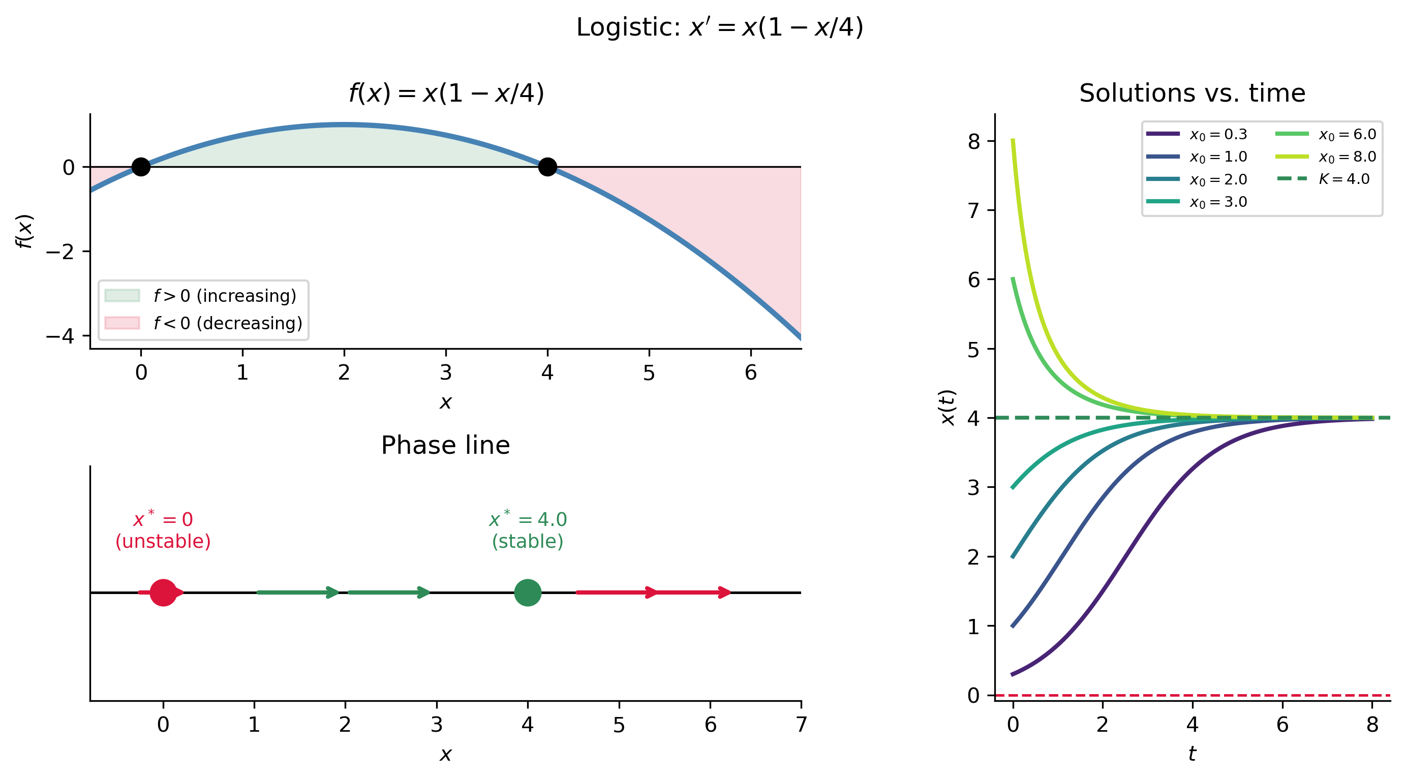
Figure 2: Phase line analysis for \(x'=x^3-x\). Left: graph of \(f(x)=x(x-1)(x+1)\) with sign regions. Middle: phase line. Right: solution curves — those starting between \(-1\) and \(1\) converge to \(x^*=0\); those outside blow up in finite time.

Linearization

Graphical phase line analysis reveals stability, but we often want an algebraic criterion. Linearization provides this.

The Linearization Criterion

Suppose \(x^*\) is an equilibrium: \(f(x^*) = 0\). Write \(x(t) = x^* + u(t)\) where \(u(t)\) is a small perturbation. Substituting into \(x' = f(x)\) and expanding \(f\) in a Taylor series about \(x^*\): \[ u' = x' = f(x^* + u) = \underbrace{f(x^*)}_{=0} + f'(x^*)\,u + \tfrac{1}{2}f''(x^*)\,u^2 + \cdots \] For small \(u\), the quadratic and higher-order terms are negligible, leaving the linearized equation: \[ u' \approx f'(x^*)\,u. \] This is a linear equation with solution \(u(t) = u(0)\,e^{f'(x^*)t}\).

ImportantLinearization Criterion (Hyperbolic Equilibria)

Let \(x^*\) be an equilibrium of \(x' = f(x)\).

  • If \(f'(x^*) < 0\): \(x^*\) is asymptotically stable (perturbations decay).
  • If \(f'(x^*) > 0\): \(x^*\) is unstable (perturbations grow).
  • If \(f'(x^*) = 0\): the test is inconclusive — higher-order terms must be examined.

An equilibrium with \(f'(x^*) \neq 0\) is called hyperbolic.

The quantity \(\lambda = f'(x^*)\) is sometimes called the eigenvalue of the equilibrium, by analogy with linear algebra.

NoteConnection to Stability and Phase Line

The linearization criterion is just an algebraic restatement of the phase line criterion: - If \(f'(x^*) < 0\), then \(f\) is decreasing through zero at \(x^*\), so \(f > 0\) just below \(x^*\) and \(f < 0\) just above — arrows point inward. - If \(f'(x^*) > 0\), then \(f\) is increasing through zero — arrows point outward.


Example 3 — Linearization Applied

Logistic equation \(x' = rx(1-x/K)\): \[ f'(x) = r\!\left(1 - \frac{2x}{K}\right). \] At \(x^* = 0\): \(f'(0) = r > 0\)unstable. At \(x^* = K\): \(f'(K) = -r < 0\)stable.

Cubic \(x' = x^3 - x\): \[ f'(x) = 3x^2 - 1. \] At \(x^* = \pm 1\): \(f'(\pm 1) = 2 > 0\)unstable. At \(x^* = 0\): \(f'(0) = -1 < 0\)stable.

Show the code
t_sym, x_sym, r_sym, K_sym = sym.symbols('t x r K', real=True, positive=True)

for label, f_expr in [
    ("Logistic $f(x)=rx(1-x/K)$",
     r_sym * x_sym * (1 - x_sym / K_sym)),
    ("Cubic $f(x)=x^3-x$",
     x_sym**3 - x_sym),
]:
    fp = sym.diff(f_expr, x_sym)
    print(f"\n{label}")
    print(f"  f'(x)  = {fp}")
    for xe, name in [(0, "x*=0"), (K_sym, "x*=K"), (1, "x*=1"), (-1, "x*=-1")]:
        try:
            val = fp.subs(x_sym, xe)
            val_s = sym.simplify(val)
            print(f"  f'({xe}) = {val_s}")
        except Exception:
            pass

Logistic $f(x)=rx(1-x/K)$
  f'(x)  = r*(1 - x/K) - r*x/K
  f'(0) = r
  f'(K) = -r
  f'(1) = r*(K - 2)/K
  f'(-1) = r*(K + 2)/K

Cubic $f(x)=x^3-x$
  f'(x)  = 3*x**2 - 1
  f'(0) = -1
  f'(K) = 3*K**2 - 1
  f'(1) = 2
  f'(-1) = 2

Example 4 — Non-Hyperbolic Equilibrium: \(x' = x^3\)

At \(x^* = 0\): \(f'(0) = 0\) — the linearization test is inconclusive. To determine stability we must look at higher-order terms. Since \(f(x) = x^3 > 0\) for \(x > 0\) and \(f(x) < 0\) for \(x < 0\), the phase line shows arrows pointing away on the left and toward on the right — the origin is semi-stable.

Show the code
f_nh  = lambda x: x**3
x_arr = np.linspace(-1.5, 1.5, 400)

fig, axes = plt.subplots(1, 2, figsize=(9, 4))

axes[0].plot(x_arr, f_nh(x_arr), color='steelblue', lw=2.5)
axes[0].axhline(0, color='k', lw=0.8)
axes[0].fill_between(x_arr, 0, f_nh(x_arr),
                     where=(f_nh(x_arr) > 0), alpha=0.15, color='crimson', label='$f>0$')
axes[0].fill_between(x_arr, 0, f_nh(x_arr),
                     where=(f_nh(x_arr) < 0), alpha=0.15, color='steelblue', label='$f<0$')
axes[0].plot(0, 0, 'ks', markersize=10, zorder=5, label='$x^*=0$ (semi-stable)')
axes[0].set_xlabel('$x$'); axes[0].set_ylabel('$f(x)$')
axes[0].set_title(r"$f(x)=x^3$: non-hyperbolic equilibrium")
axes[0].legend(fontsize=8)

f_ode_nh = lambda t, x: [x[0]**3]
t_eval = np.linspace(0, 2, 400)
for x0, color in zip([-1.2, -0.7, -0.3, 0.3, 0.7, 1.2],
                     plt.cm.RdBu(np.linspace(0.05, 0.95, 6))):
    sol = solve_ivp(f_ode_nh, (0, 1.8), [x0], t_eval=np.linspace(0,1.8,400),
                    max_step=0.005, events=lambda t,y: abs(y[0])-8)
    axes[1].plot(sol.t, np.clip(sol.y[0], -5, 5), color=color, lw=2, label=f'$x_0={x0}$')
axes[1].axhline(0, color='k', ls='--', lw=1.5, label='$x^*=0$')
axes[1].set_xlabel('$t$'); axes[1].set_ylabel('$x(t)$')
axes[1].set_title('Semi-stable: solutions above blow up, below approach 0')
axes[1].legend(fontsize=7, ncol=2); axes[1].set_ylim(-4, 4)

plt.tight_layout()
plt.show()
Figure 3: Non-hyperbolic equilibrium \(x'=x^3\) at \(x^*=0\). The linearization \(f'(0)=0\) is inconclusive. The full phase line reveals semi-stability: solutions above \(x^*=0\) move away, solutions below approach.

Bifurcations

What Is a Bifurcation?

In many models, the ODE \(x' = f(x; r)\) contains a parameter \(r\) (a growth rate, a temperature, a control voltage). As \(r\) varies, the equilibria may appear, disappear, or change stability. A bifurcation is a qualitative change in the equilibrium structure at a critical parameter value \(r = r_c\), called the bifurcation point.

ImportantDefinition: Bifurcation

A value \(r = r_c\) is a bifurcation point of \(x' = f(x; r)\) if the number or stability of equilibria changes as \(r\) passes through \(r_c\).

A bifurcation diagram plots the equilibrium values \(x^*\) as a function of \(r\), using a solid curve for stable equilibria and a dashed curve for unstable ones. It provides a complete summary of the system’s parameter-dependent behavior in a single picture.

We study three classical bifurcations: saddle-node, transcritical, and pitchfork.


The Saddle-Node Bifurcation

The saddle-node bifurcation (also called a fold bifurcation) is the most generic way that equilibria are created or destroyed. The normal form is: \[ x' = r - x^2. \]

Equilibria: \(r - x^2 = 0 \Rightarrow x^* = \pm\sqrt{r}\) (real only when \(r \geq 0\)).

Linearization: \(f'(x) = -2x\). At \(x^* = +\sqrt{r}\): \(f'= -2\sqrt{r} < 0\)stable. At \(x^* = -\sqrt{r}\): \(f' = +2\sqrt{r} > 0\)unstable.

Parameter Equilibria Character
\(r < 0\) None No equilibria
\(r = 0\) \(x^* = 0\) One semi-stable equilibrium (bifurcation point)
\(r > 0\) \(x^* = \pm\sqrt{r}\) Two equilibria: stable (\(+\)) and unstable (\(-\))

A stable and an unstable equilibrium collide and annihilate as \(r\) decreases through zero.

Show the code
fig, axes = plt.subplots(1, 3, figsize=(13, 4.5))

# f(x) for three r values
x_arr = np.linspace(-2.2, 2.2, 400)
colors3 = ['crimson', 'darkorange', 'steelblue']
for r_val, color, lbl in zip([-0.5, 0, 1.0], colors3, ['$r=-0.5$','$r=0$','$r=1$']):
    axes[0].plot(x_arr, r_val - x_arr**2, color=color, lw=2, label=lbl)
axes[0].axhline(0, color='k', lw=0.8)
axes[0].set_xlabel('$x$'); axes[0].set_ylabel('$f(x) = r - x^2$')
axes[0].set_title('$f(x)$ for three values of $r$')
axes[0].legend(fontsize=9); axes[0].set_ylim(-2, 2)

# Phase lines
ax_pl = axes[1]
y_offsets = {'$r=-0.5$': -0.7, '$r=0$': 0.0, '$r=1$': 0.7}
for r_val, color, lbl in zip([-0.5, 0, 1.0], colors3, ['$r=-0.5$','$r=0$','$r=1$']):
    y0 = y_offsets[lbl]
    ax_pl.axhline(y0, color=color, lw=1.2, alpha=0.6)
    ax_pl.text(-2.0, y0+0.07, lbl, fontsize=8, color=color)
    if r_val < 0:
        for xm in [-1.5, 0.0, 1.5]:
            sign = -1 if r_val - xm**2 < 0 else 1
            ax_pl.annotate('', xy=(xm + 0.25*sign, y0),
                           xytext=(xm, y0),
                           arrowprops=dict(arrowstyle='->', color=color, lw=1.5))
    elif r_val == 0:
        ax_pl.plot(0, y0, 's', color=color, markersize=10, zorder=5)
        for xm in [-1.5, 1.5]:
            sign = -1 if -xm**2 < 0 else 1
            ax_pl.annotate('', xy=(xm + 0.25*sign, y0),
                           xytext=(xm, y0),
                           arrowprops=dict(arrowstyle='->', color=color, lw=1.5))
    else:
        xe_s =  np.sqrt(r_val)
        xe_u = -np.sqrt(r_val)
        ax_pl.plot(xe_s, y0, 'o', color='steelblue', markersize=10, zorder=5)
        ax_pl.plot(xe_u, y0, 'o', color='crimson',   markersize=10, zorder=5,
                   markerfacecolor='white', markeredgewidth=2)
        for xm in [-1.8, 0.0]:
            sign = -1 if r_val - xm**2 < 0 else 1
            ax_pl.annotate('', xy=(xm + 0.25*sign, y0),
                           xytext=(xm, y0),
                           arrowprops=dict(arrowstyle='->', color=color, lw=1.5))
        ax_pl.annotate('', xy=(xe_s+0.3, y0), xytext=(xe_s+0.05, y0),
                       arrowprops=dict(arrowstyle='<-', color=color, lw=1.5))
ax_pl.set_xlim(-2.2, 2.2); ax_pl.set_ylim(-1.1, 1.1)
ax_pl.set_xlabel('$x$'); ax_pl.set_yticks([])
ax_pl.set_title('Phase lines')

# Bifurcation diagram
r_bif  = np.linspace(-0.05, 2.5, 400)
r_pos  = r_bif[r_bif >= 0]
axes[2].plot(r_pos,  np.sqrt(r_pos),  color='steelblue', lw=2.5, label='Stable ($x^*=+\\sqrt{r}$)')
axes[2].plot(r_pos, -np.sqrt(r_pos),  color='crimson',   lw=2.5, ls='--', label='Unstable ($x^*=-\\sqrt{r}$)')
axes[2].plot(0, 0, 'ko', markersize=8, zorder=5, label='Bifurcation point')
axes[2].set_xlabel('Parameter $r$'); axes[2].set_ylabel('Equilibrium $x^*$')
axes[2].set_title('Bifurcation diagram')
axes[2].legend(fontsize=8); axes[2].axvline(0, color='k', lw=0.5, ls=':')

plt.suptitle('Saddle-Node Bifurcation: $x\'=r-x^2$', fontsize=12)
plt.tight_layout()
plt.show()
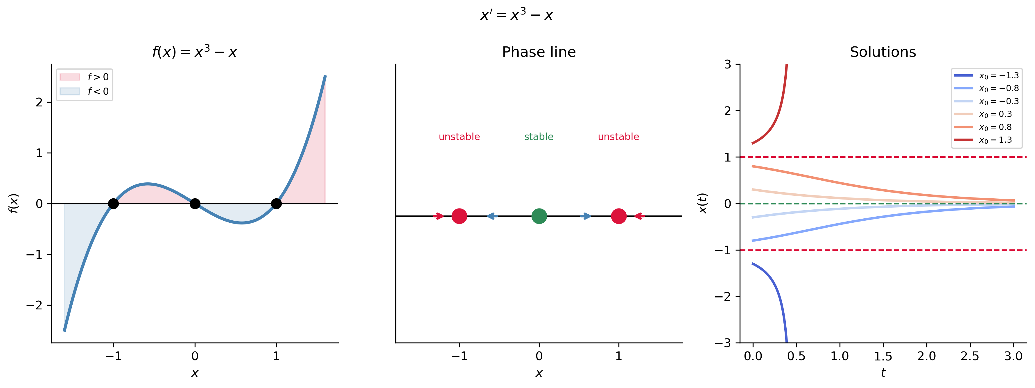
Figure 4: Saddle-node bifurcation \(x'=r-x^2\). Left: \(f(x)\) for three values of \(r\). Middle: phase lines for each case. Right: bifurcation diagram — stable branch (solid blue) and unstable branch (dashed red) emerge from the bifurcation point \(r=0\).

The Transcritical Bifurcation

The transcritical bifurcation occurs when two equilibria exist for all values of \(r\) but exchange stability at the bifurcation point. The normal form is: \[ x' = rx - x^2 = x(r - x). \]

Equilibria: \(x^* = 0\) and \(x^* = r\) for all \(r\).

Linearization: \(f'(x) = r - 2x\). So \(f'(0) = r\) and \(f'(r) = -r\).

\(r\) \(x^*=0\) \(x^*=r\)
\(r < 0\) Stable (\(f'(0)=r<0\)) Unstable (\(f'(r)=-r>0\))
\(r = 0\) Non-hyperbolic (Same point)
\(r > 0\) Unstable (\(f'(0)=r>0\)) Stable (\(f'(r)=-r<0\))

The two equilibria swap stability as \(r\) passes through zero. This bifurcation arises naturally in population models where \(x=0\) is always an equilibrium: the trivial (zero-population) state loses stability when \(r\) crosses a threshold, and a non-trivial population \(x^*=r\) becomes the attractor.

Show the code
fig, axes = plt.subplots(1, 2, figsize=(10, 4.5))

# f(x) plots
x_arr = np.linspace(-1.5, 3.0, 400)
for r_val, color, lbl in zip([-0.8, 0.0, 1.2],
                              ['crimson', 'darkorange', 'steelblue'],
                              ['$r=-0.8$', '$r=0$', '$r=1.2$']):
    axes[0].plot(x_arr, r_val*x_arr - x_arr**2, color=color, lw=2, label=lbl)
axes[0].axhline(0, color='k', lw=0.8)
axes[0].set_xlabel('$x$'); axes[0].set_ylabel('$f(x)=rx-x^2$')
axes[0].set_title('$f(x)$ for several $r$')
axes[0].legend(fontsize=9); axes[0].set_ylim(-2, 1)

# Bifurcation diagram
r_bif = np.linspace(-1.5, 2.5, 400)
# x*=0: stable for r<0 (solid), unstable for r>0 (dashed)
axes[1].plot(r_bif[r_bif <= 0], np.zeros(np.sum(r_bif<=0)),
             color='steelblue', lw=2.5, label='$x^*=0$ stable')
axes[1].plot(r_bif[r_bif >= 0], np.zeros(np.sum(r_bif>=0)),
             color='steelblue', lw=2.5, ls='--', label='$x^*=0$ unstable')
# x*=r: unstable for r<0 (dashed), stable for r>0 (solid)
axes[1].plot(r_bif[r_bif <= 0], r_bif[r_bif <= 0],
             color='crimson', lw=2.5, ls='--', label='$x^*=r$ unstable')
axes[1].plot(r_bif[r_bif >= 0], r_bif[r_bif >= 0],
             color='crimson', lw=2.5, label='$x^*=r$ stable')
axes[1].plot(0, 0, 'ko', markersize=8, zorder=5, label='Bifurcation point')
axes[1].set_xlabel('Parameter $r$'); axes[1].set_ylabel('Equilibrium $x^*$')
axes[1].set_title('Bifurcation diagram')
axes[1].legend(fontsize=8, ncol=2)
axes[1].axvline(0, color='k', lw=0.5, ls=':')

plt.suptitle(r"Transcritical Bifurcation: $x'=rx-x^2$", fontsize=12)
plt.tight_layout()
plt.show()
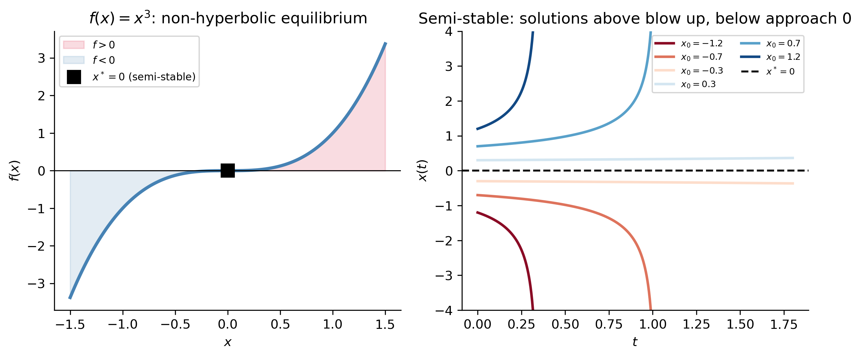
Figure 5: Transcritical bifurcation \(x'=rx-x^2\). The two equilibria \(x^*=0\) and \(x^*=r\) exist for all \(r\) and exchange stability at \(r=0\).

The Pitchfork Bifurcation

The pitchfork bifurcation arises in systems with a symmetry (\(f(-x;r) = -f(x;r)\)). A single equilibrium at the origin loses or gains stability, accompanied by the creation of a symmetric pair of equilibria.

Supercritical Pitchfork

The supercritical pitchfork normal form is: \[ x' = rx - x^3. \]

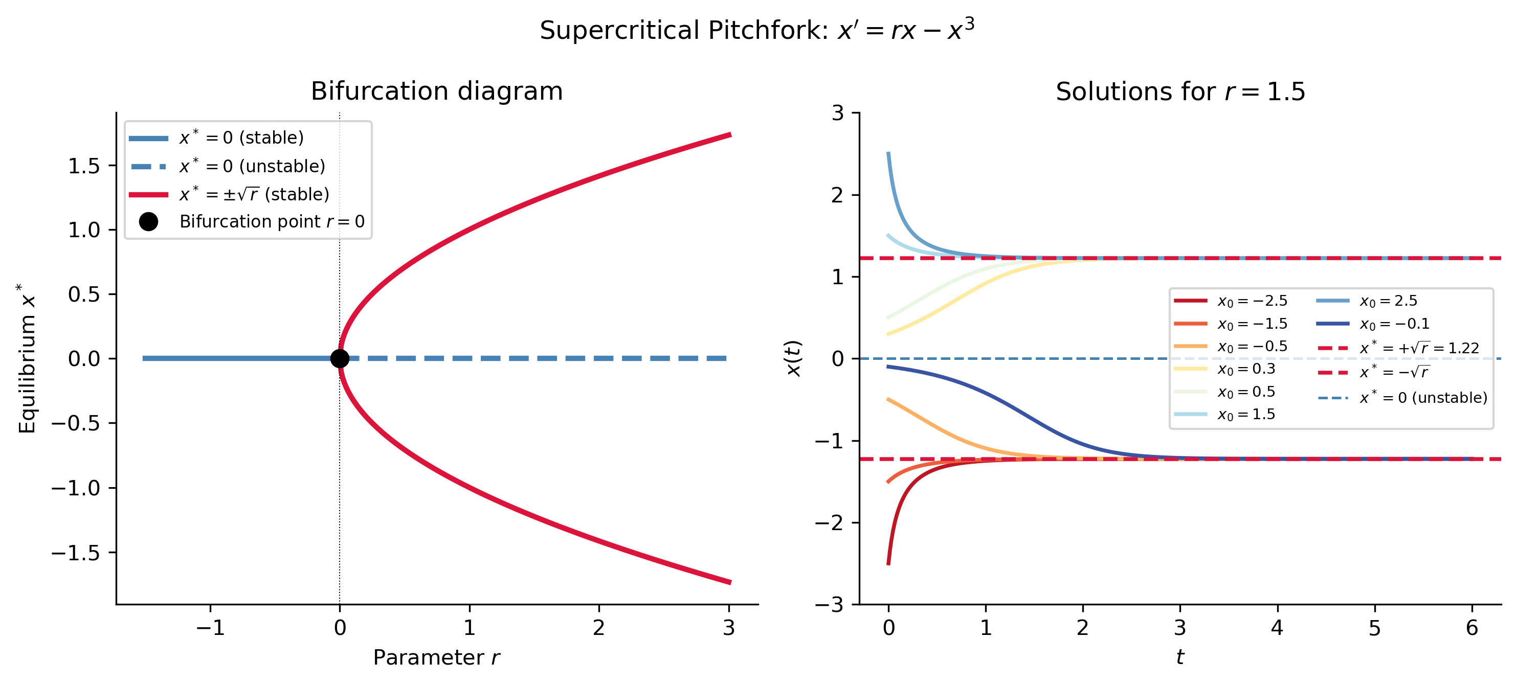
Equilibria: \(x(r - x^2) = 0 \Rightarrow x^* = 0\) always; \(x^* = \pm\sqrt{r}\) when \(r > 0\).

Linearization: \(f'(x) = r - 3x^2\).

\(r \leq 0\) \(x^*=0\) stable (\(f'(0)=r\leq 0\)) No other equilibria
\(r > 0\) \(x^*=0\) unstable (\(f'(0)=r>0\)) \(x^*=\pm\sqrt{r}\) stable (\(f'(\pm\sqrt{r})=-2r<0\))

As \(r\) increases through zero, the stable origin loses stability and two new stable equilibria bifurcate symmetrically. The bifurcation diagram has the shape of a pitchfork.

Show the code
fig, axes = plt.subplots(1, 2, figsize=(10, 4.5))

# Bifurcation diagram
r_bif = np.linspace(-1.5, 3.0, 400)
# x*=0: stable for r<0 (solid), unstable for r>0 (dashed)
axes[0].plot(r_bif[r_bif <= 0], np.zeros(np.sum(r_bif <= 0)),
             color='steelblue', lw=2.5, label='$x^*=0$ (stable)')
axes[0].plot(r_bif[r_bif >= 0], np.zeros(np.sum(r_bif >= 0)),
             color='steelblue', lw=2.5, ls='--', label='$x^*=0$ (unstable)')
# x*=±sqrt(r) for r>0: stable
r_pos = r_bif[r_bif >= 0]
axes[0].plot(r_pos,  np.sqrt(r_pos), color='crimson', lw=2.5, label=r'$x^*=\pm\sqrt{r}$ (stable)')
axes[0].plot(r_pos, -np.sqrt(r_pos), color='crimson', lw=2.5)
axes[0].plot(0, 0, 'ko', markersize=8, zorder=5, label='Bifurcation point $r=0$')
axes[0].set_xlabel('Parameter $r$'); axes[0].set_ylabel('Equilibrium $x^*$')
axes[0].set_title('Bifurcation diagram')
axes[0].legend(fontsize=8); axes[0].axvline(0, color='k', lw=0.5, ls=':')

# Solution curves for r=1.5
r_fixed = 1.5
xe_stable = np.sqrt(r_fixed)
f_pf = lambda t, x: [r_fixed*x[0] - x[0]**3]
t_eval = np.linspace(0, 6, 400)
colors_pf = plt.cm.RdYlBu(np.linspace(0.05, 0.95, 8))
for x0, color in zip([-2.5,-1.5,-0.5, 0.3, 0.5, 1.5, 2.5, -0.1],
                      colors_pf):
    sol = solve_ivp(f_pf, (0,6), [x0], t_eval=t_eval, max_step=0.02)
    axes[1].plot(sol.t, sol.y[0], color=color, lw=1.8, label=f'$x_0={x0}$')
axes[1].axhline( xe_stable, color='crimson',  ls='--', lw=1.8, label=f'$x^*=+\\sqrt{{r}}={xe_stable:.2f}$')
axes[1].axhline(-xe_stable, color='crimson',  ls='--', lw=1.8, label=f'$x^*=-\\sqrt{{r}}$')
axes[1].axhline(0,          color='steelblue', ls='--', lw=1.2, label='$x^*=0$ (unstable)')
axes[1].set_xlabel('$t$'); axes[1].set_ylabel('$x(t)$')
axes[1].set_title(f'Solutions for $r={r_fixed}$')
axes[1].legend(fontsize=7, ncol=2); axes[1].set_ylim(-3, 3)

plt.suptitle(r"Supercritical Pitchfork: $x'=rx-x^3$", fontsize=12)
plt.tight_layout()
plt.show()
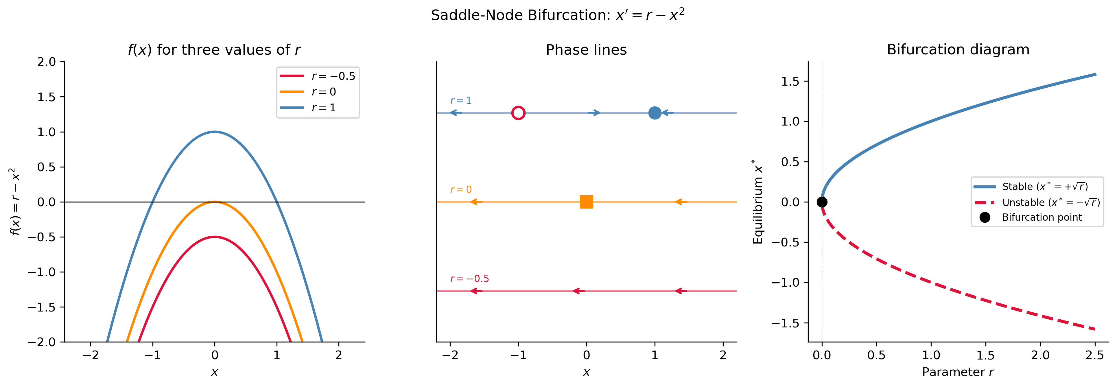
Figure 6: Supercritical pitchfork bifurcation \(x'=rx-x^3\). Left: bifurcation diagram — the stable origin loses stability at \(r=0\) and two symmetric stable branches emerge. Right: solution curves for \(r=1.5\) showing all trajectories converging to one of the two stable equilibria \(\pm\sqrt{r}\).

Subcritical Pitchfork

The subcritical pitchfork normal form is: \[ x' = rx + x^3. \] Now for \(r < 0\) there are three equilibria (\(x^*=0\) stable, \(x^*=\pm\sqrt{-r}\) unstable), and for \(r \geq 0\) only \(x^* = 0\) exists and is unstable. The bifurcation is “dangerous” because when \(r\) crosses zero from below, all equilibria disappear simultaneously and solutions blow up.

TipSupercritical vs. Subcritical
  • Supercritical (\(x'=rx-x^3\)): new stable equilibria born as \(r\) increases through zero — a smooth, “soft” transition. Encountered in phase transitions, buckling, and symmetry breaking.
  • Subcritical (\(x'=rx+x^3\)): unstable equilibria exist below the bifurcation and disappear at the critical point — a “hard” or dangerous transition with no warning.

Summary: The Three Classic Bifurcations

Show the code
fig, axes = plt.subplots(1, 3, figsize=(13, 4))

# Saddle-node: x' = r - x^2
r = np.linspace(-0.2, 2.0, 300)
r_pos = r[r >= 0]
axes[0].plot(r_pos,  np.sqrt(r_pos), color='steelblue', lw=2.5, label='Stable')
axes[0].plot(r_pos, -np.sqrt(r_pos), color='crimson',   lw=2.5, ls='--', label='Unstable')
axes[0].plot(0, 0, 'ko', markersize=8)
axes[0].axvline(0, color='k', lw=0.5, ls=':')
axes[0].set_xlabel('$r$'); axes[0].set_ylabel('$x^*$')
axes[0].set_title("Saddle-Node\n$x'=r-x^2$")
axes[0].legend(fontsize=8)

# Transcritical: x' = rx - x^2
r2 = np.linspace(-1.5, 2.0, 300)
axes[1].plot(r2[r2<=0], np.zeros(np.sum(r2<=0)), color='steelblue', lw=2.5)
axes[1].plot(r2[r2>=0], np.zeros(np.sum(r2>=0)), color='steelblue', lw=2.5, ls='--')
axes[1].plot(r2[r2<=0], r2[r2<=0], color='crimson', lw=2.5, ls='--')
axes[1].plot(r2[r2>=0], r2[r2>=0], color='crimson', lw=2.5)
axes[1].plot(0, 0, 'ko', markersize=8)
axes[1].axvline(0, color='k', lw=0.5, ls=':')
axes[1].set_xlabel('$r$'); axes[1].set_ylabel('$x^*$')
axes[1].set_title("Transcritical\n$x'=rx-x^2$")

# Pitchfork: x' = rx - x^3
r3 = np.linspace(-1.5, 2.5, 300)
r3_pos = r3[r3 >= 0]
axes[2].plot(r3[r3<=0], np.zeros(np.sum(r3<=0)), color='steelblue', lw=2.5)
axes[2].plot(r3[r3>=0], np.zeros(np.sum(r3>=0)), color='steelblue', lw=2.5, ls='--')
axes[2].plot(r3_pos,  np.sqrt(r3_pos), color='crimson', lw=2.5)
axes[2].plot(r3_pos, -np.sqrt(r3_pos), color='crimson', lw=2.5, label='Stable branches')
axes[2].plot(0, 0, 'ko', markersize=8)
axes[2].axvline(0, color='k', lw=0.5, ls=':')
axes[2].set_xlabel('$r$'); axes[2].set_ylabel('$x^*$')
axes[2].set_title("Pitchfork (supercritical)\n$x'=rx-x^3$")
axes[2].legend(fontsize=8)

for ax in axes:
    ax.axhline(0, color='k', lw=0.5)

plt.tight_layout()
plt.show()
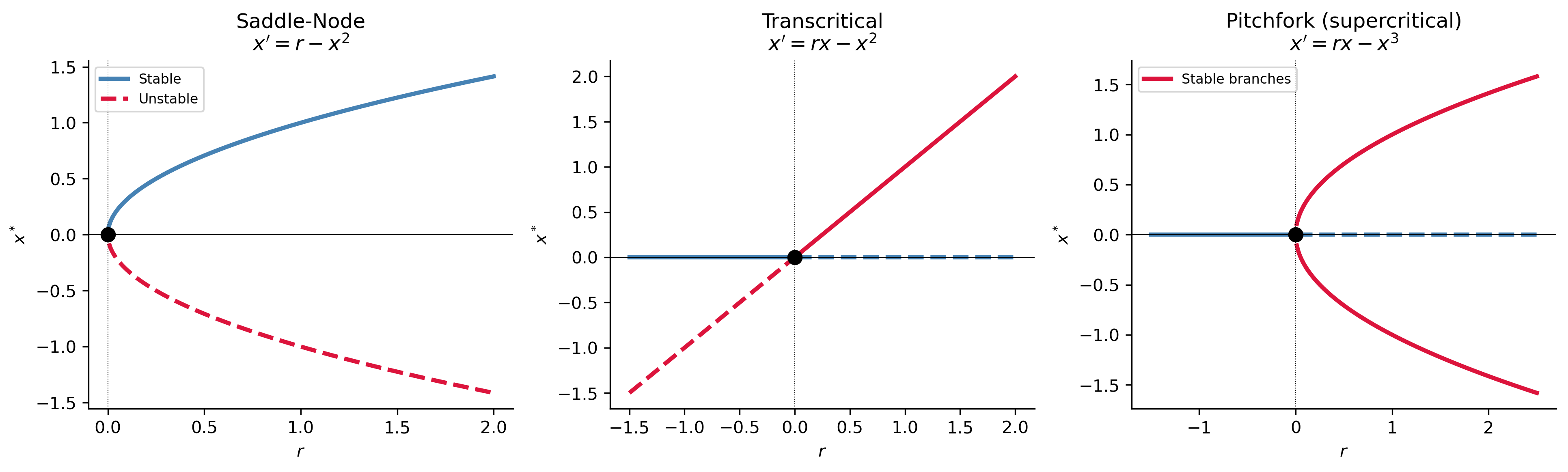
Figure 7: Bifurcation diagrams for all three classical one-dimensional bifurcations. Solid curves are stable equilibria; dashed curves are unstable. The bifurcation point in each case is at \(r=0\).

Application: The Spruce Budworm Model

A classical ecological bifurcation occurs in the spruce budworm model, proposed by Ludwig, Jones, and Holling (1978). The dimensionless form is: \[ x' = rx\!\left(1 - \frac{x}{K}\right) - \frac{x^2}{1+x^2}, \] where \(x\) is the budworm population density, \(r\) is the growth rate, \(K\) is the carrying capacity, and the last term is a predation function (Type III functional response).

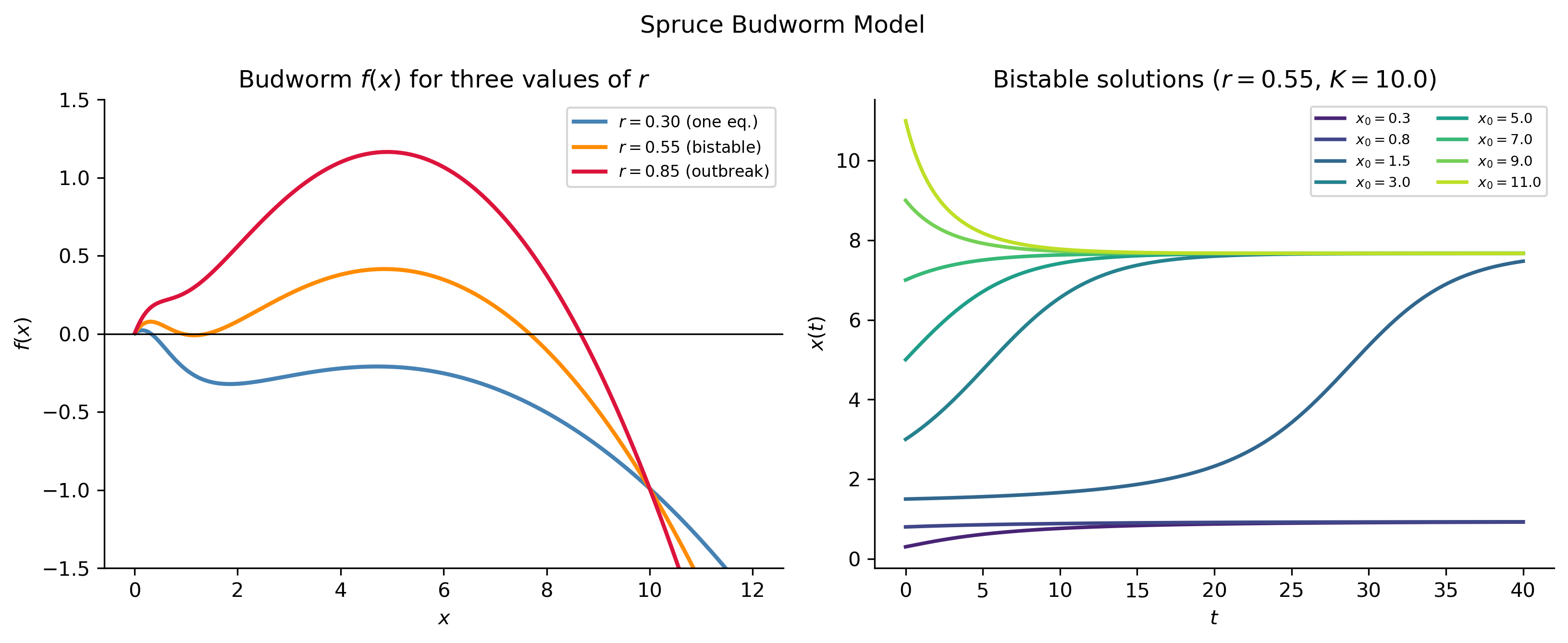
The system can exhibit bistability: for certain parameter values there are two stable equilibria — a low “refuge” state and a high “outbreak” state — separated by an unstable one. This leads to hysteresis: the system can jump suddenly from refuge to outbreak state when \(r\) crosses a critical threshold, and will not return to refuge unless \(r\) is reduced well below the forward bifurcation point.

Show the code
K_bw = 10.0

fig, axes = plt.subplots(1, 2, figsize=(11, 4.5))

# f(x) for three r values
x_arr = np.linspace(0.01, 12, 400)
pred  = x_arr**2 / (1 + x_arr**2)
for r_val, color, lbl in zip([0.3, 0.55, 0.85],
                               ['steelblue', 'darkorange', 'crimson'],
                               ['$r=0.30$ (one eq.)', '$r=0.55$ (bistable)', '$r=0.85$ (outbreak)']):
    growth = r_val * x_arr * (1 - x_arr/K_bw)
    axes[0].plot(x_arr, growth - pred, color=color, lw=2, label=lbl)
axes[0].axhline(0, color='k', lw=0.8)
axes[0].set_xlabel('$x$'); axes[0].set_ylabel('$f(x)$')
axes[0].set_title('Budworm $f(x)$ for three values of $r$')
axes[0].legend(fontsize=8); axes[0].set_ylim(-1.5, 1.5)

# Solutions for bistable case r=0.55
r_bw  = 0.55
f_bw  = lambda t, x: [r_bw*x[0]*(1-x[0]/K_bw) - x[0]**2/(1+x[0]**2)]
t_eval = np.linspace(0, 40, 600)
for x0, color in zip([0.3, 0.8, 1.5, 3.0, 5.0, 7.0, 9.0, 11.0],
                     plt.cm.viridis(np.linspace(0.1, 0.9, 8))):
    sol = solve_ivp(f_bw, (0, 40), [x0], t_eval=t_eval, max_step=0.05)
    axes[1].plot(sol.t, sol.y[0], color=color, lw=1.8, label=f'$x_0={x0}$')
axes[1].set_xlabel('$t$'); axes[1].set_ylabel('$x(t)$')
axes[1].set_title(f'Bistable solutions ($r={r_bw}$, $K={K_bw}$)')
axes[1].legend(fontsize=7, ncol=2)

plt.suptitle("Spruce Budworm Model", fontsize=12)
plt.tight_layout()
plt.show()
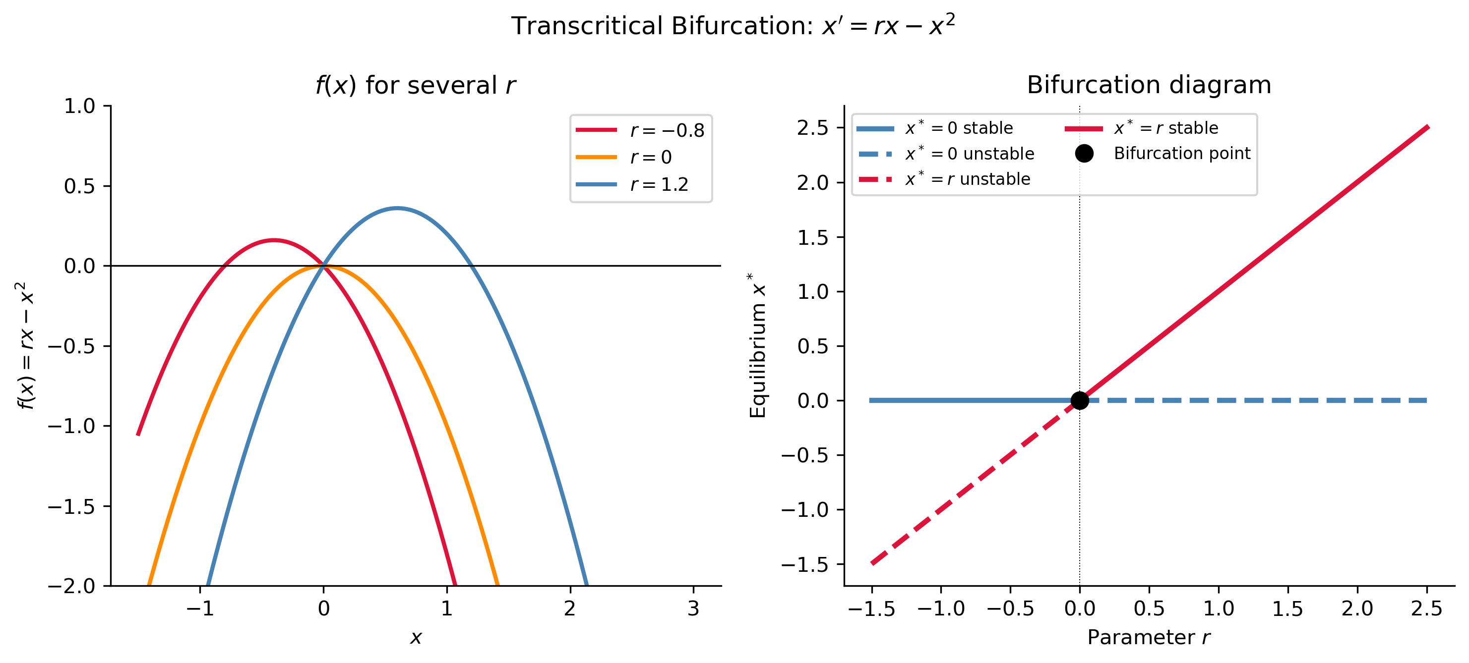
Figure 8: Spruce budworm model with \(K=10\). Left: \(f(x)\) for three values of \(r\), showing how the number of positive equilibria changes. Right: solutions from multiple initial conditions for the bistable case (\(r=0.55\)) — the population converges to either the low refuge state or the high outbreak state depending on the initial condition.

Summary

Concept Key Idea
Autonomous ODE \(x'=f(x)\): slope depends only on state, not time
Equilibrium \(x^*\) with \(f(x^*)=0\); constant solution
Stable equilibrium Nearby solutions converge to \(x^*\); \(f'(x^*)<0\)
Unstable equilibrium Nearby solutions diverge from \(x^*\); \(f'(x^*)>0\)
Phase line Arrows determined by sign of \(f(x)\); complete qualitative picture
Linearization \(u'\approx f'(x^*)u\); stability from sign of \(f'(x^*)\)
Bifurcation Qualitative change in equilibrium structure as parameter varies
Saddle-node Creation/annihilation of a stable–unstable pair
Transcritical Two equilibria exchange stability
Pitchfork Symmetric birth of two new equilibria; supercritical (soft) or subcritical (hard)
TipLooking Ahead

The ideas introduced here — equilibria, stability, and bifurcations — extend directly to systems of ODEs in two and higher dimensions. Equilibria of two-dimensional systems are classified by the eigenvalues of the Jacobian matrix (the analog of \(f'(x^*)\)), and the phase plane replaces the phase line. Bifurcations in two dimensions include the Hopf bifurcation, where a stable equilibrium gives birth to a stable limit cycle (sustained oscillation). These topics are covered in Chapter 3 of Logan (2015).


These notes are also viewable as a slide deck presentation: Open slides in full screen

Note

Next: Second-order linear equations — Logan §2.2.


Relevant Videos

Autonomous ODEs, Equilibria, and Stability:

Phase-Line Diagrams:

Bifurcation Diagrams:

References

Logan, J David. 2015. A First Course in Differential Equations Third Edition.
Show the code
import sys
print("Python version:", sys.version)
print('\n'.join(f'{m.__name__}=={m.__version__}' for m in globals().values() if getattr(m, '__version__', None)))
Python version: 3.14.4 | packaged by conda-forge | (main, Apr  8 2026, 02:33:53) [Clang 20.1.8 ]
numpy==2.4.3
sympy==1.14.0
matplotlib==3.10.8