Notes 14

Numerical Methods for Differential Equations

Show the code
import numpy as np
import matplotlib as mpl
import matplotlib.pyplot as plt
from scipy.integrate import solve_ivp
from IPython.display import display, Math, Image
mpl.rcParams['figure.dpi'] = 150
mpl.rcParams['axes.spines.top']   = False
mpl.rcParams['axes.spines.right'] = False

Goals

In this section, we will:

  1. Understand why numerical methods are indispensable — most differential equations arising in science and engineering cannot be solved analytically, and even those that can are often more usefully studied numerically.

  2. Derive the Euler method (6.5) from a first-order Taylor expansion and interpret it geometrically as “stepping along the slope field.”

  3. Understand the local truncation error \(O(h^2)\) and the global (cumulative) error \(O(h)\) for the Euler method, and verify the \(O(h)\) convergence rate numerically.

  4. Derive the modified Euler method (predictor–corrector, second-order Runge–Kutta) and understand why its global error is \(O(h^2)\).

  5. State the fourth-order Runge–Kutta (RK4) update formula and its four slope evaluations \(k_1, k_2, k_3, k_4\), giving a global error \(O(h^4)\).

  6. Extend all three methods to systems of ODEs (§6.3), writing out the Euler, modified Euler, and RK4 update formulas for the two-dimensional system \(x' = f(t,x,y)\), \(y' = g(t,x,y)\).

  7. Use scipy.integrate.solve_ivp as a practical tool for solving IVPs, selecting solvers, controlling tolerances, and interpreting results.

Note

This material corresponds to Sections 6.2 and 6.3 of (Logan 2015).


Why Numerical Methods?

Most differential equations cannot be solved analytically by a simple formula. In industry and science, differential equations are almost always solved numerically because most real-world models lead to models too complicated to solve analytically. And, in the rare case that the problem can be solved analytically, the solution is often in the form of a complicated integral or infinite series which must be resolved by a computer calculation anyway. Logan remarks that “many would say that the material in this brief section is the most important in the entire book.”

The goal is this: given the IVP

\[ x' = f(t, x), \qquad x(t_0) = x_0, \tag{6.3} \]

produce a sequence of approximations \(X_0, X_1, X_2, \ldots, X_N\) at discrete times \(t_0 < t_1 < \cdots < t_N = T\), connected by straight line segments, that accurately represents the true solution \(x(t)\).


Section 6.2 — Numerical Methods

Discretization

We divide the interval \([t_0, T]\) into \(N\) equal subintervals of length

\[ h = \frac{T - t_0}{N} \qquad (\text{the \textbf{step size}}), \]

defining the equally-spaced grid

\[ t_n = t_0 + nh, \quad n = 0, 1, 2, \ldots, N. \]

We seek a recursive formula that computes \(X_{n+1}\) from \(X_n\). Starting from \(X_0 = x_0\), this formula is applied \(N\) times to march from \(t_0\) to \(T\), yielding the numerical solution \(\{(t_n, X_n)\}\).


Section 6.2.1 — The Euler Method

Derivation

Integrate the ODE \(x'(t) = f(t, x(t))\) from \(t_n\) to \(t_{n+1}\):

\[ \int_{t_n}^{t_{n+1}} x'(t)\,dt = \int_{t_n}^{t_{n+1}} f(t, x(t))\,dt. \tag{6.4} \]

The left side equals \(x(t_{n+1}) - x(t_n)\) by the Fundamental Theorem. The right side is approximated by the left-hand (rectangle) rule: replace \(f(t, x(t))\) by its value at the left endpoint \(t_n\):

\[ x(t_{n+1}) - x(t_n) = h\,f(t_n, x(t_n)) + O(h^2). \]

Neglecting the \(O(h^2)\) term and writing \(X_n\) for the approximation of \(x(t_n)\):

ImportantThe Euler Method

\[ X_{n+1} = X_n + h\,f(t_n, X_n), \quad n = 0, 1, 2, \ldots, N, \tag{6.5} \] with \(X_0 = x_0\).

Geometric Interpretation

At each step, the Euler method draws the tangent line to the solution curve at \((t_n, X_n)\), which lies in the direction of the slope field, and follows it for a distance \(h\) to obtain \(X_{n+1}\). It is an explicit method — \(X_{n+1}\) is computed directly from \(X_n\) with no equation to solve.

Error Analysis

  • Local truncation error: \(O(h^2)\) per step (error introduced in approximating one integral).
  • Global (cumulative) error: \(O(h)\) over the whole interval (since there are \(N = (T-t_0)/h\) steps, \(N \cdot O(h^2) = O(h)\)). Euler’s method is said to be first-order accurate.
  • Consequence: halving \(h\) approximately halves the global error.

Visualizing the Euler Method

The animation below shows the Euler method applied to \(x' = t - x\), \(x(0) = 1\) with \(h = 0.25\). At each step: the green segment shows the Euler step (following the local slope); the orange bracket shows the local error (gap between the approximate and exact values).

Euler method animation: \(x'=t-x\), \(x(0)=1\), \(h=0.25\). The green segment at each step follows the slope field; the orange bracket shows the growing gap between the numerical approximation (red) and the exact solution (blue).

Example 6.3 — Euler Method by Hand

Solve \(x' = t - x\), \(x(0) = 1\) on \([0, 2]\) with \(N = 8\) steps (\(h = 0.25\)). Here \(f(t,x) = t - x\) and \(t_n = 0.25n\). The Euler recurrence is

\[ X_{n+1} = X_n + 0.25(t_n - X_n) = X_n + 0.25(0.25n - X_n). \]

Starting with \(X_0 = 1\):

\[ X_1 = 1 + 0.25(0 - 1) = 0.75, \quad X_2 = 0.75 + 0.25(0.25 - 0.75) = 0.625. \]

Continuing: \(X_3 = 0.594\), \(X_4 = 0.632\), \(\ldots\), \(X_7 = 1.017\), \(X_8 = 1.200\).

The exact solution (by integrating factor) is \(x(t) = t - 1 + 2e^{-t}\), giving \(x(2) = 1.2707\).

Show the code
def f_ex(t, x):
    return t - x

def euler(f, t0, T, x0, N):
    h = (T - t0) / N
    t = np.linspace(t0, T, N+1)
    X = np.zeros(N+1); X[0] = x0
    for n in range(N):
        X[n+1] = X[n] + h * f(t[n], X[n])
    return t, X

def exact_ex(t):
    return t - 1 + 2*np.exp(-t)

t0, T, x0 = 0.0, 2.0, 1.0
t_fine = np.linspace(t0, T, 400)

fig, ax = plt.subplots(figsize=(9, 5))
ax.plot(t_fine, exact_ex(t_fine), 'steelblue', lw=2.8, label='Exact $x(t)=t-1+2e^{-t}$')

colors = ['crimson', 'darkorange', 'seagreen']
Nvals  = [4, 8, 16]
hvals  = [(T-t0)/N for N in Nvals]

for N, color, h in zip(Nvals, colors, hvals):
    t_e, X_e = euler(f_ex, t0, T, x0, N)
    err = abs(exact_ex(T) - X_e[-1])
    ax.plot(t_e, X_e, color=color, lw=1.8, marker='o', markersize=5,
            label=f'Euler $h={h}$, error at $t=2$: {err:.4f}')

ax.set_xlabel('$t$'); ax.set_ylabel('$x$')
ax.set_title("Example 6.3: Euler method convergence")
ax.legend(fontsize=9)
plt.tight_layout()
plt.show()

# Error table
print(f"{'h':>8}  {'X(2)':>8}  {'error':>8}")
print("-" * 28)
for N, h in zip(Nvals, hvals):
    _, X_e = euler(f_ex, t0, T, x0, N)
    err = exact_ex(T) - X_e[-1]
    print(f"{h:8.4f}  {X_e[-1]:8.4f}  {err:8.4f}")
print(f"{'exact':>8}  {exact_ex(T):8.4f}  {'0':>8}")
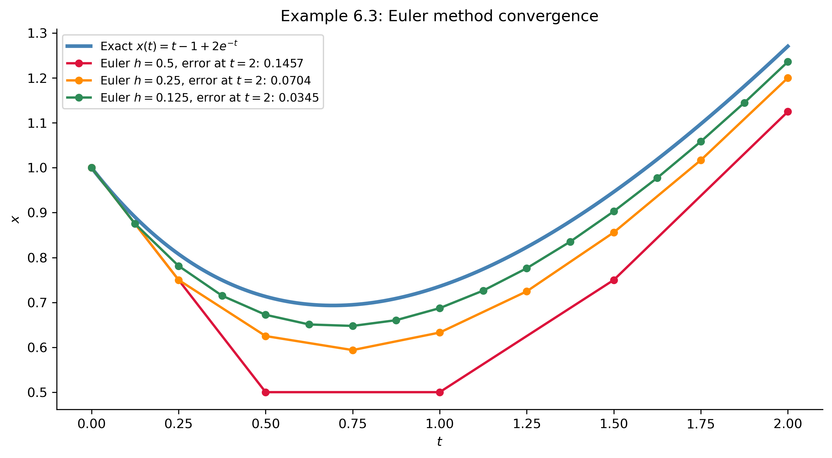
Figure 1: Example 6.3 — Euler method applied to \(x'=t-x\), \(x(0)=1\) with step sizes \(h=0.5, 0.25, 0.125\) (red, orange, green), compared to the exact solution \(x(t)=t-1+2e^{-t}\) (blue). Each approximation lags behind the exact solution (which is concave up). Error at \(t=2\) is approximately halved each time \(h\) is halved, confirming \(O(h)\) convergence.
       h      X(2)     error
----------------------------
  0.5000    1.1250    0.1457
  0.2500    1.2002    0.0704
  0.1250    1.2361    0.0345
   exact    1.2707         0

The Modified Euler Method (Second-Order Runge–Kutta)

To improve accuracy, replace the left-hand rectangle rule in (6.4) with the trapezoidal rule:

\[ x(t_{n+1}) - x(t_n) = \frac{h}{2}\bigl[f(t_n, x(t_n)) + f(t_{n+1}, x(t_{n+1}))\bigr] + O(h^3). \]

This gives a local truncation error of \(O(h^3)\) and a global error of \(O(h^2)\). The formula (6.6) involves \(X_{n+1}\) on both sides (an implicit equation), making it expensive to solve at each step.

The practical fix is a predictor–corrector approach:

ImportantModified Euler Method (RK2)

Predictor (Euler step): \[\widetilde{X}_{n+1} = X_n + h\,f(t_n, X_n). \tag{6.7}\]

Corrector (trapezoidal average): \[X_{n+1} = X_n + \frac{h}{2}\bigl[f(t_n, X_n) + f(t_{n+1}, \widetilde{X}_{n+1})\bigr]. \tag{6.8}\]

Global error: \(O(h^2)\). Also called the second-order Runge–Kutta method.

The new value \(X_{n+1}\) is the average of the slope at the current point and the (predicted) slope at the next point.


Section 6.2.2 — The Fourth-Order Runge–Kutta Method (RK4)

The most widely used algorithm for numerical ODEs is the classical fourth-order Runge–Kutta method, which achieves a global error of \(O(h^4)\). It evaluates \(f\) at four carefully chosen points within each interval:

ImportantThe Runge–Kutta Method (RK4)

\[ X_{n+1} = X_n + \frac{h}{6}(k_1 + 2k_2 + 2k_3 + k_4), \] where \[ k_1 = f(t_n,\; X_n), \quad k_2 = f\!\left(t_n + \tfrac{h}{2},\; X_n + \tfrac{h}{2}k_1\right), \] \[ k_3 = f\!\left(t_n + \tfrac{h}{2},\; X_n + \tfrac{h}{2}k_2\right), \quad k_4 = f(t_n + h,\; X_n + h\,k_3). \] The new value is a weighted average of four slopes \(k_1, \ldots, k_4\) sampled at the left endpoint, two midpoints, and the right endpoint.

Error Comparison

The table below shows theoretical error orders and concrete computed errors for \(x' = t - x\), \(x(0) = 1\), comparing the error at \(t = 2\) for two step sizes. The exact answer is \(x(2) = 1.27067\ldots\)

Method Order Error (\(h=0.5\)) Error (\(h=0.25\)) Ratio
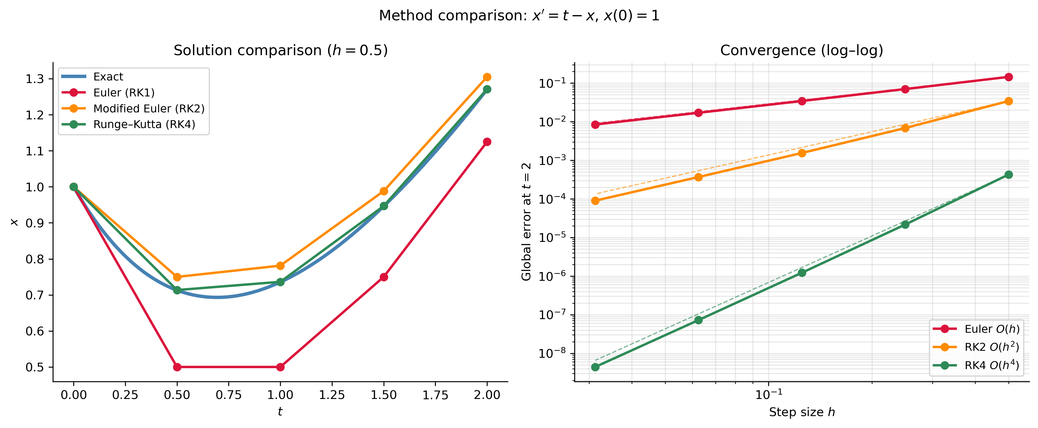
Euler \(O(h)\) \(0.1457\) \(0.0704\) \(2.07\approx 2^1\)
Modified Euler (RK2) \(O(h^2)\) \(0.0107\) \(0.0027\) \(3.96\approx 2^2\)
Runge–Kutta (RK4) \(O(h^4)\) \(0.0000540\) \(0.0000034\) \(15.9\approx 2^4\)

The Ratio column confirms the theoretical orders: halving \(h\) approximately halves the error for Euler (\(\times 2\)), quarters it for RK2 (\(\times 4\)), and reduces it by a factor of 16 for RK4 (\(\times 16 = 2^4\)). This dramatic difference is why RK4 is the standard choice when accuracy matters.

Show the code
def modified_euler(f, t0, T, x0, N):
    h = (T - t0) / N
    t = np.linspace(t0, T, N+1)
    X = np.zeros(N+1); X[0] = x0
    for n in range(N):
        Xt = X[n] + h * f(t[n], X[n])
        X[n+1] = X[n] + (h/2) * (f(t[n], X[n]) + f(t[n+1], Xt))
    return t, X

def rk4(f, t0, T, x0, N):
    h = (T - t0) / N
    t = np.linspace(t0, T, N+1)
    X = np.zeros(N+1); X[0] = x0
    for n in range(N):
        k1 = f(t[n],       X[n])
        k2 = f(t[n]+h/2,   X[n]+h/2*k1)
        k3 = f(t[n]+h/2,   X[n]+h/2*k2)
        k4 = f(t[n]+h,     X[n]+h*k3)
        X[n+1] = X[n] + (h/6)*(k1 + 2*k2 + 2*k3 + k4)
    return t, X

fig, axes = plt.subplots(1, 2, figsize=(12, 5))

# Left: solution comparison with h=0.5
N_demo = 4
t_fine = np.linspace(0, 2, 400)
axes[0].plot(t_fine, exact_ex(t_fine), 'steelblue', lw=2.8,
             label='Exact')
for method, color, lbl in [
        (euler,          'crimson',    'Euler (RK1)'),
        (modified_euler, 'darkorange', 'Modified Euler (RK2)'),
        (rk4,            'seagreen',   'Runge–Kutta (RK4)')]:
    t_m, X_m = method(f_ex, 0, 2, 1, N_demo)
    axes[0].plot(t_m, X_m, marker='o', markersize=6, lw=2.0,
                 color=color, label=lbl)
axes[0].set_xlabel('$t$'); axes[0].set_ylabel('$x$')
axes[0].set_title('Solution comparison ($h=0.5$)')
axes[0].legend(fontsize=9)

# Right: convergence log-log
h_vals = [0.5, 0.25, 0.125, 0.0625, 0.03125]
for method, color, lbl, order in [
        (euler,          'crimson',    'Euler $O(h)$',    1),
        (modified_euler, 'darkorange', 'RK2 $O(h^2)$',   2),
        (rk4,            'seagreen',   'RK4 $O(h^4)$',   4)]:
    errs = []
    for h in h_vals:
        N_ = int(2/h)
        _, X_m = method(f_ex, 0, 2, 1, N_)
        errs.append(abs(exact_ex(2) - X_m[-1]))
    axes[1].loglog(h_vals, errs, marker='o', color=color, lw=2.0, label=lbl)
    # Reference slope
    h_arr = np.array(h_vals)
    axes[1].loglog(h_arr, errs[0]*(h_arr/h_vals[0])**order,
                   ls='--', color=color, lw=1.0, alpha=0.6)

axes[1].set_xlabel('Step size $h$'); axes[1].set_ylabel('Global error at $t=2$')
axes[1].set_title('Convergence (log–log)')
axes[1].legend(fontsize=9)
axes[1].grid(True, which='both', alpha=0.3)

plt.suptitle(r"Method comparison: $x'=t-x$, $x(0)=1$", fontsize=12)
plt.tight_layout()
plt.show()
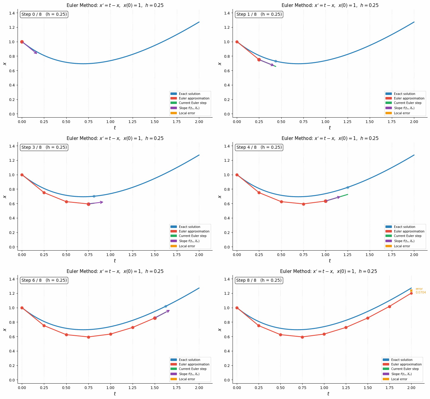
Figure 2: Comparison of Euler (red), Modified Euler/RK2 (orange), and RK4 (green) with \(h=0.5\) on \(x'=t-x\), \(x(0)=1\). Even with this large step size, RK4 is almost indistinguishable from the exact solution. The right panel shows convergence: log–log plot of global error at \(t=2\) vs. \(h\) confirms slopes of 1, 2, and 4 for Euler, RK2, and RK4.
Show the code
# Verify the concrete error table values above (all method functions now defined)
_methods = [('Euler', euler), ('Modified Euler (RK2)', modified_euler), ('RK4', rk4)]
print(f"{'Method':<24} {'h=0.5 error':>12} {'h=0.25 error':>13} {'Ratio':>7}")
print("-" * 60)
for name, method in _methods:
    err_half    = abs(exact_ex(2) - method(f_ex, 0, 2, 1,  4)[-1][-1])
    err_quarter = abs(exact_ex(2) - method(f_ex, 0, 2, 1,  8)[-1][-1])
    ratio = err_half / err_quarter
    print(f"{name:<24} {err_half:>12.7f} {err_quarter:>13.7f} {ratio:>7.2f}")
Method                    h=0.5 error  h=0.25 error   Ratio
------------------------------------------------------------
Euler                       0.1456706     0.0704447    2.07
Modified Euler (RK2)        0.0345052     0.0068852    5.01
RK4                         0.0004290     0.0000217   19.75

Error Sources

There are three sources of error in a finite difference scheme:

  1. Truncation error — arises from approximating the continuous problem by a discrete one (Taylor series truncation). This is the \(O(h^p)\) error analyzed above.

  2. Stability error — the discrete algorithm itself may be unstable: an error at an early step can be amplified as it propagates forward in time. The step size \(h\) must be kept below a problem-dependent threshold.

  3. Roundoff error — a computer represents real numbers with finite precision. The actual computed value \(\overline{X}_n\) differs from the mathematically exact discrete value \(X_n\) by the roundoff error \(X_n - \overline{X}_n\).

The total error at \(t_n\) is

\[ x(t_n) - \overline{X}_n = \underbrace{(x(t_n) - X_n)}_{\text{truncation}} + \underbrace{(X_n - \overline{X}_n)}_{\text{roundoff}}. \]

Visual Exploration of Methods

To help develop our intuition for these numerical methods, let’s view this visual web app.

NoteStiff Equations

Some differential equations are stiff: they have components that change at vastly different time scales. Simple slope-following methods like Euler and even RK4 require extremely small step sizes to remain stable on stiff problems. Stiff solvers (e.g., backward Euler, implicit Runge–Kutta) are required; scipy provides these via the method='Radau' or method='BDF' options in solve_ivp.


Section 6.3 — Numerical Methods for Systems

The single-equation methods extend immediately to the two-dimensional system

\[ x' = f(t, x, y), \qquad y' = g(t, x, y), \]

with initial conditions \(x(t_0) = x_0\), \(y(t_0) = y_0\). We write \(X_n \approx x(t_n)\) and \(Y_n \approx y(t_n)\).

Euler Method for Systems

\[ X_{n+1} = X_n + h\,f(t_n, X_n, Y_n), \] \[ Y_{n+1} = Y_n + h\,g(t_n, X_n, Y_n). \]

Modified Euler Method for Systems

Predictors: \[\widetilde{X}_{n+1} = X_n + h\,f(t_n, X_n, Y_n), \qquad \widetilde{Y}_{n+1} = Y_n + h\,g(t_n, X_n, Y_n).\]

Correctors: \[X_{n+1} = X_n + \frac{h}{2}\bigl[f(t_n, X_n, Y_n) + f(t_{n+1}, \widetilde{X}_{n+1}, \widetilde{Y}_{n+1})\bigr],\] \[Y_{n+1} = Y_n + \frac{h}{2}\bigl[g(t_n, X_n, Y_n) + g(t_{n+1}, \widetilde{X}_{n+1}, \widetilde{Y}_{n+1})\bigr].\]

Runge–Kutta Method for Systems

Compute eight slopes at each step:

\[ k_{11} = f(t_n, X_n, Y_n), \quad k_{21} = g(t_n, X_n, Y_n), \] \[ k_{12} = f\!\left(t_n+\tfrac{h}{2},\; X_n+\tfrac{h}{2}k_{11},\; Y_n+\tfrac{h}{2}k_{21}\right), \quad k_{22} = g\!\left(t_n+\tfrac{h}{2},\; X_n+\tfrac{h}{2}k_{11},\; Y_n+\tfrac{h}{2}k_{21}\right), \] \[ k_{13} = f\!\left(t_n+\tfrac{h}{2},\; X_n+\tfrac{h}{2}k_{12},\; Y_n+\tfrac{h}{2}k_{22}\right), \quad k_{23} = g\!\left(t_n+\tfrac{h}{2},\; X_n+\tfrac{h}{2}k_{12},\; Y_n+\tfrac{h}{2}k_{22}\right), \] \[ k_{14} = f(t_n+h,\; X_n+hk_{13},\; Y_n+hk_{23}), \quad k_{24} = g(t_n+h,\; X_n+hk_{13},\; Y_n+hk_{23}). \]

Then:

\[ X_{n+1} = X_n + \frac{h}{6}(k_{11} + 2k_{12} + 2k_{13} + k_{14}), \] \[ Y_{n+1} = Y_n + \frac{h}{6}(k_{21} + 2k_{22} + 2k_{23} + k_{24}). \]

The global errors remain order \(h\), \(h^2\), and \(h^4\) for Euler, modified Euler, and RK4, respectively. The procedure extends in the same way to systems of any dimension.


Using scipy.integrate.solve_ivp

Why Use solve_ivp?

Rather than programming the methods above from scratch (which is valuable for understanding), in practice we use scipy.integrate.solve_ivp, which:

  • Implements high-quality, adaptive step-size methods that automatically tighten \(h\) where the solution changes rapidly and relax it where it is smooth.
  • Provides multiple solvers: 'RK45' (default, explicit 4th/5th-order), 'RK23', 'DOP853', 'Radau' (stiff), 'BDF' (stiff), 'LSODA'.
  • Returns a rich result object with solution values, time points, success/failure status, and optionally a dense interpolant.

Basic Usage

from scipy.integrate import solve_ivp

# Define the right-hand side: must accept (t, y) where y is a 1-D array
def rhs(t, y):
    return [t - y[0]]       # y[0] is x(t)

# Solve
sol = solve_ivp(
    fun     = rhs,          # right-hand side f(t, y)
    t_span  = (0, 2),       # integration interval [t0, T]
    y0      = [1.0],        # initial condition (list or array)
    method  = 'RK45',       # solver (default; adaptive 4th/5th-order RK)
    dense_output = True,    # enable continuous interpolant sol.sol(t)
    rtol    = 1e-6,         # relative tolerance
    atol    = 1e-8,         # absolute tolerance
)

print(f"Success: {sol.success}")
print(f"Solver steps taken: {len(sol.t)}")
print(f"x(2) ≈ {sol.y[0, -1]:.8f}  (exact: {exact_ex(2):.8f})")

# Plot using the dense interpolant
t_plot = np.linspace(0, 2, 400)
x_interp = sol.sol(t_plot)[0]   # shape (1, 400) → take row 0

fig, ax = plt.subplots(figsize=(8, 4))
ax.plot(t_plot, exact_ex(t_plot), 'steelblue', lw=2.5, label='Exact')
ax.plot(t_plot, x_interp, 'seagreen', lw=2.0, ls='--', label='solve_ivp RK45')
ax.plot(sol.t, sol.y[0], 'go', markersize=5,
        label=f'Adaptive steps (N={len(sol.t)})')
ax.set_xlabel('$t$'); ax.set_ylabel('$x(t)$')
ax.set_title(r"$x'=t-x$, $x(0)=1$ via `solve_ivp`")
ax.legend(fontsize=9)
plt.tight_layout()
plt.show()
Success: True
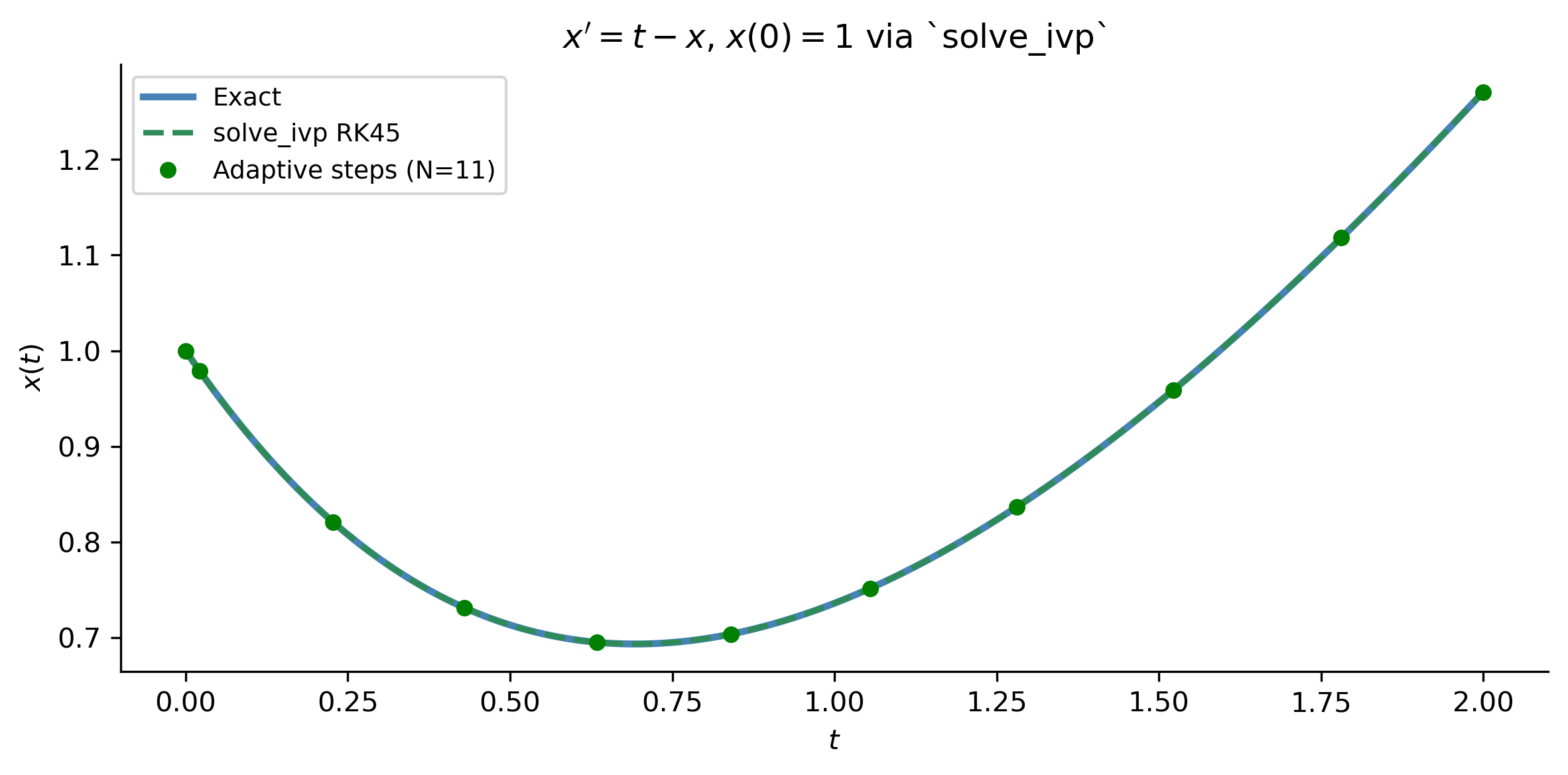
Solver steps taken: 11
x(2) ≈ 1.27067069  (exact: 1.27067057)
Figure 3: Solving \(x'=t-x\), \(x(0)=1\) with solve_ivp using default RK45 (green circles) and a fixed fine grid (dense_output=True). The result is essentially indistinguishable from the exact solution (blue).

Solving Systems with solve_ivp

For a system, simply stack the state variables into a vector and define the right-hand side accordingly:

# Lotka-Volterra: x' = ax - bxy,  y' = -cy + dxy
a, b, c, d = 0.6, 0.5, 0.3, 0.4

def lv_rhs(t, z):
    x, y = z
    return [a*x - b*x*y,
            -c*y + d*x*y]

sol_lv = solve_ivp(
    fun          = lv_rhs,
    t_span       = (0, 60),
    y0           = [c/d + 0.4, a/b],   # perturbed from equilibrium
    method       = 'RK45',
    dense_output = True,
    rtol         = 1e-9,
    atol         = 1e-11,
    max_step     = 0.05,
)

t_p = np.linspace(0, 60, 1500)
z_p = sol_lv.sol(t_p)

fig, axes = plt.subplots(1, 2, figsize=(11, 4.5))

axes[0].plot(t_p, z_p[0], 'steelblue', lw=2.5, label='$x(t)$ prey')
axes[0].plot(t_p, z_p[1], 'crimson',   lw=2.5, label='$y(t)$ predator')
axes[0].axhline(c/d, color='steelblue', ls=':', lw=1, alpha=0.7)
axes[0].axhline(a/b, color='crimson',   ls=':', lw=1, alpha=0.7)
axes[0].set_xlabel('$t$'); axes[0].set_ylabel('Population')
axes[0].set_title('Lotka–Volterra time series')
axes[0].legend(fontsize=9)

axes[1].plot(z_p[0], z_p[1], 'seagreen', lw=1.8)
axes[1].plot(c/d, a/b, 'o', color='steelblue', markersize=9,
             label=f'Equilibrium $({c/d:.2f},{a/b:.2f})$')
axes[1].set_xlabel('$x$ (prey)'); axes[1].set_ylabel('$y$ (predator)')
axes[1].set_title('Phase portrait')
axes[1].legend(fontsize=9)

plt.suptitle(f'Lotka–Volterra ($a={a}$, $b={b}$, $c={c}$, $d={d}$)', fontsize=11)
plt.tight_layout()
plt.show()
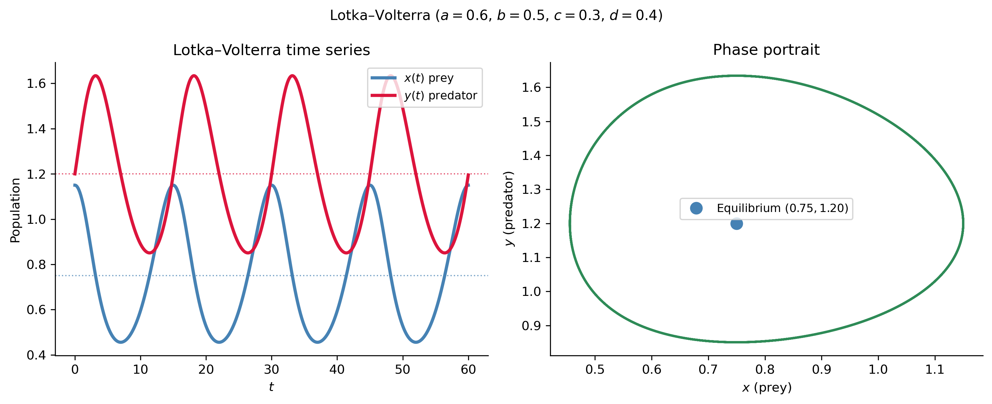
Figure 4: Lotka–Volterra predator–prey system solved with solve_ivp. Left: time series of prey \(x(t)\) (steelblue) and predator \(y(t)\) (crimson) showing the classic antiphase oscillations. Right: phase portrait showing the closed orbit around the non-trivial equilibrium, confirming the periodic nature of the solution.

Key solve_ivp Options

Option Purpose Typical value
method Solver algorithm 'RK45' (default), 'Radau' (stiff)
t_eval Times at which to store solution np.linspace(t0, T, 500)
dense_output Enable sol.sol(t) interpolant True
rtol Relative tolerance 1e-6 (default 1e-3)
atol Absolute tolerance 1e-8 (default 1e-6)
max_step Upper bound on step size Useful for periodic problems
events Detect zero-crossings Function returning scalar
TipChoosing a Solver
  • Non-stiff problems (most problems in this course): 'RK45' (default) is excellent.
  • Stiff problems (large Jacobian eigenvalue spread): use 'Radau' or 'BDF'.
  • High accuracy needed: 'DOP853' (8th-order explicit).
  • When in doubt: try 'RK45' first. If it is slow or fails to converge, switch to 'Radau'.

Summary

Method Formula Global error Evaluations/step
Euler \(X_{n+1}=X_n+hf(t_n,X_n)\) \(O(h)\) 1
Modified Euler (RK2) Predictor (6.7) + Corrector (6.8) \(O(h^2)\) 2
Runge–Kutta (RK4) Weighted avg of \(k_1,k_2,k_3,k_4\) \(O(h^4)\) 4
solve_ivp RK45 Adaptive embedded pair \(O(h^5)\), auto-\(h\) varies

All three methods extend to systems by treating \((X_n, Y_n)\) as a vector and applying the scalar formula component-wise. The global error orders \(O(h)\), \(O(h^2)\), \(O(h^4)\) are unchanged.

TipLooking Ahead

The methods in this section — particularly RK4 and solve_ivp — are the tools used throughout numerical science and engineering. They underlie every phase portrait produced in Chapters 4 and 5 of Logan, all the nonlinear systems analyzed in Chapter 5, and the time-series solutions for models in biology, chemistry, and physics. Understanding why these methods work, not just how to call them, is the lasting take-away from this chapter.


These notes are also viewable as a slide deck presentation: Open slides in full screen

Note

Next: Review and additional computational topics.


Relevant Videos

Numerical Methods for ODEs — Overview:

The Euler Method:

Runge–Kutta Methods:

The Euler Method for Systems:

scipy.integrate.solve_ivp Tutorial:

References

Logan, J David. 2015. A First Course in Differential Equations, Third Edition.
Show the code
import sys
print("Python version:", sys.version)
print('\n'.join(f'{m.__name__}=={m.__version__}' for m in globals().values() if getattr(m, '__version__', None)))
Python version: 3.14.4 | packaged by conda-forge | (main, Apr  8 2026, 02:33:53) [Clang 20.1.8 ]
numpy==2.4.3
matplotlib==3.10.8