Variation of Parameters for Second-Order Linear ODEs
Show the code
import numpy as npimport sympy as symimport matplotlib as mplimport matplotlib.pyplot as pltfrom scipy.integrate import solve_ivpfrom IPython.display import Math, displaympl.rcParams['figure.dpi'] =150mpl.rcParams['axes.spines.top'] =Falsempl.rcParams['axes.spines.right'] =False
Note
Estimated reading time: 55–70 minutes
Goals
In this section we will:
State the general theory for second-order linear ODEs with variable coefficients and explain when the method of undetermined coefficients fails.
Develop the method of variation of parameters as a general technique for finding particular solutions — applicable to any second-order linear ODE, including those with variable coefficients.
Work through a suite of detailed examples, including equations with trigonometric, exponential, and rational forcing functions, as well as an Euler equation with variable-coefficient homogeneous part.
Use SymPy and Python to verify solutions and visualize particular solutions alongside their homogeneous counterparts.
Note
This material corresponds to Section 2.4.2 of (Logan 2015).
NoteConnection to Notes 4
In Notes 4 we introduced variation of parameters as one of two methods for finding particular solutions of constant-coefficient equations, alongside undetermined coefficients. Here we develop the method more fully: we derive the formula from scratch, prove when it applies, work through four detailed examples (including the Euler equation, which has variable coefficients), and clarify exactly when to prefer it over undetermined coefficients. If you used variation of parameters in Notes 4, everything here will be familiar in structure — the new content is the generality and the examples.
Variable-Coefficient Second-Order ODEs
The General Equation
A second-order linear ODE with variable coefficients has the form \[
p(t)\,x'' + q(t)\,x' + r(t)\,x = f(t), \tag{VC}
\] where the coefficient functions \(p(t)\), \(q(t)\), \(r(t)\) and the forcing function \(f(t)\) are continuous on some interval \(I\), with \(p(t) \neq 0\) on \(I\). Dividing by \(p(t)\) puts the equation in standard form: \[
x'' + P(t)\,x' + Q(t)\,x = g(t), \tag{SF}
\] where \(P = q/p\), \(Q = r/p\), and \(g = f/p\).
The Superposition Principle and the general solution structure\(x = x_h + x_p\) hold for (SF) exactly as for the constant-coefficient case. What changes is the method we use to find \(x_h\) and \(x_p\), since the exponential ansatz \(e^{\lambda t}\) no longer works when the coefficients vary.
When Undetermined Coefficients Fails
The method of undetermined coefficients requires the right-hand side \(g(t)\) to be a polynomial, exponential, sine, cosine, or product thereof. For variable-coefficient equations the homogeneous solution \(x_h\) no longer consists of these simple forms, so there is no longer a predictable guess for \(x_p\). Moreover, even for constant-coefficient equations, forcing functions such as \(\sec t\), \(\tan t\), \(\ln t\), \(1/t\), or \(e^t/t\) lie outside the undetermined-coefficients table and cannot be handled by guessing.
Not in the guess table; derivatives generate new function families
\(\ln t\), \(\sqrt{t}\), \(1/t\)
Not closed under differentiation — infinitely many new terms appear
\(e^t/t\)
Product of an exponential and \(1/t\); \(1/t\) grows under differentiation
Variable coefficients
No exponential \(x_h\) to compare against; guessing is not predictable
Variation of parameters handles all of these by working directly with the homogeneous solutions, whatever form they take.
The Method of Variation of Parameters
Derivation
Suppose we know two linearly independent solutions \(x_1(t)\) and \(x_2(t)\) of the homogeneous equation \[
x'' + P(t)\,x' + Q(t)\,x = 0. \tag{H}
\] Their general solution is \(x_h = C_1 x_1 + C_2 x_2\). In variation of parameters, we allow the constants to vary: seek a particular solution of the form \[
x_p(t) = u_1(t)\,x_1(t) + u_2(t)\,x_2(t)
\] where \(u_1(t)\) and \(u_2(t)\) are functions to be determined.
Computing \(x_p'\):\[
x_p' = u_1'x_1 + u_1 x_1' + u_2'x_2 + u_2 x_2'.
\] We impose the side condition\[
u_1'x_1 + u_2'x_2 = 0 \tag{SC}
\] to eliminate second derivatives of \(u_1\), \(u_2\) when we differentiate again. This gives \(x_p' = u_1 x_1' + u_2 x_2'\) and \[
x_p'' = u_1'x_1' + u_1 x_1'' + u_2'x_2' + u_2 x_2''.
\]Substituting into (SF) and using the fact that \(x_1\), \(x_2\) satisfy (H): \[
u_1'x_1' + u_2'x_2' = g(t). \tag{D}
\] Equations (SC) and (D) form the \(2\times 2\) linear system for \(u_1'\) and \(u_2'\): \[
\begin{pmatrix} x_1 & x_2 \\ x_1' & x_2' \end{pmatrix}
\begin{pmatrix} u_1' \\ u_2' \end{pmatrix}
=
\begin{pmatrix} 0 \\ g(t) \end{pmatrix}.
\] The coefficient matrix is the Wronskian matrix whose determinant \[
W(x_1, x_2) = x_1 x_2' - x_2 x_1'
\] If this is non-zero, we can solve the system by Cramer’s rule: \[
u_1' = -\frac{x_2\,g}{W}, \qquad u_2' = \frac{x_1\,g}{W}.
\] Integrating: \[
u_1 = -\int\frac{x_2\,g}{W}\,dt, \qquad u_2 = \int\frac{x_1\,g}{W}\,dt.
\]
ImportantVariation of Parameters Formula
Given two linearly independent solutions \(x_1\), \(x_2\) of (H) with Wronskian \(W = x_1 x_2' - x_2 x_1'\), a particular solution of \(x'' + Px' + Qx = g\) is \[
\boxed{x_p(t) = -x_1(t)\int\frac{x_2(t)\,g(t)}{W(t)}\,dt \;+\; x_2(t)\int\frac{x_1(t)\,g(t)}{W(t)}\,dt.}
\] The general solution is \(x(t) = C_1 x_1(t) + C_2 x_2(t) + x_p(t)\).
Abel’s Identity
The Wronskian of any two solutions of (H) satisfies Abel’s identity: \[
W(t) = W(t_0)\,\exp\!\left(-\int_{t_0}^t P(s)\,ds\right).
\] For constant-coefficient equations (\(P\) constant) this gives \(W(t) = W(t_0)\,e^{-P(t-t_0)}\), and in particular \(W \neq 0\) everywhere if it is non-zero at one point. More generally, since the exponential factor is always nonzero, Abel’s identity shows that \(W\) either vanishes identically on \(I\) or is nonzero everywhere on \(I\) — in particular, if \(W(t_0)\neq 0\) for any single \(t_0\in I\), then \(W(t)\neq 0\) for all \(t\in I\). This justifies checking the Wronskian at just one convenient point.
Step-by-Step Procedure
ImportantAlgorithm for Variation of Parameters
Write the ODE in standard form:\(x'' + P(t)x' + Q(t)x = g(t)\).
Find \(x_1\), \(x_2\): two linearly independent solutions of the homogeneous equation.
Compute the Wronskian:\(W = x_1 x_2' - x_2 x_1'\).
General solution:\[\boxed{x(t) = C_1\cos t + C_2\sin t + \cos t\ln|\cos t| + t\sin t.}\]
Note
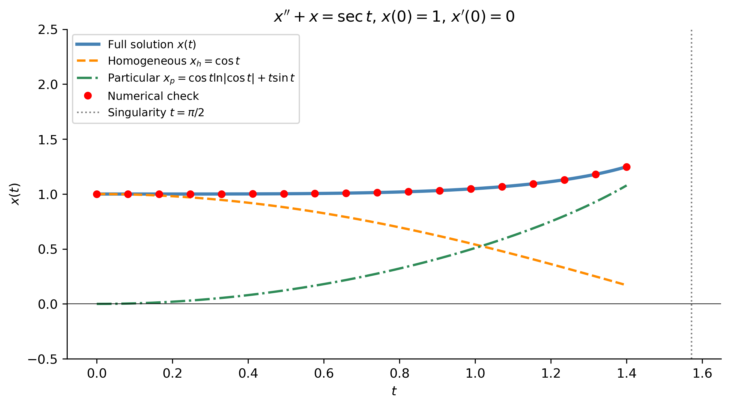
The solution exists on the interval \((-\pi/2,\,\pi/2)\) containing \(t=0\), and more generally on any open interval between consecutive singularities of \(\sec t\) (i.e., between adjacent odd multiples of \(\pi/2\)). The \(t\sin t\) term in \(x_p\) causes the amplitude to grow linearly — behavior analogous to resonance, even though \(\omega = 1\) and the forcing \(\sec t\) is not a pure sinusoid. Undetermined coefficients never produces this kind of growth.
Figure 1: Example 1: \(x''+x=\sec t\), \(x(0)=1\), \(x'(0)=0\) (solved on \([0,\pi/2)\) before the singularity). The full solution (blue) is the sum of the homogeneous part (orange dashed) and the particular solution \(x_p=\cos t\ln|\cos t|+t\sin t\) (green). Red dots confirm the analytical formula via numerical ODE solve.
Example 2 — \(x'' - 2x' + x = e^t/t\)
This equation has a repeated eigenvalue — the homogeneous solutions are \(x_1 = e^t\) and \(x_2 = te^t\), and the forcing \(e^t/t\) is outside the undetermined-coefficients table (the \(1/t\) factor makes it inadmissible).
Step 1. Already in standard form; \(g(t) = e^t/t\).
Step 6.\[x_p = e^t\cdot(-t) + te^t\cdot\ln t = te^t(\ln t - 1).\]
General solution:\[\boxed{x(t) = C_1 e^t + C_2 te^t + te^t(\ln t - 1), \quad t > 0.}\]
Note
Note that \(te^t(\ln t - 1) = te^t\ln t - te^t\), and the \(-te^t\) part could be absorbed into the \(C_2 te^t\) term by redefining \(C_2\). This is valid because particular solutions are not unique — any particular solution differs from any other by a solution of the homogeneous equation, so absorbing constant-multiple terms from \(x_p\) into \(x_h\) yields the same general solution. In practice we keep the particular solution as found and let the constants adjust when ICs are applied.
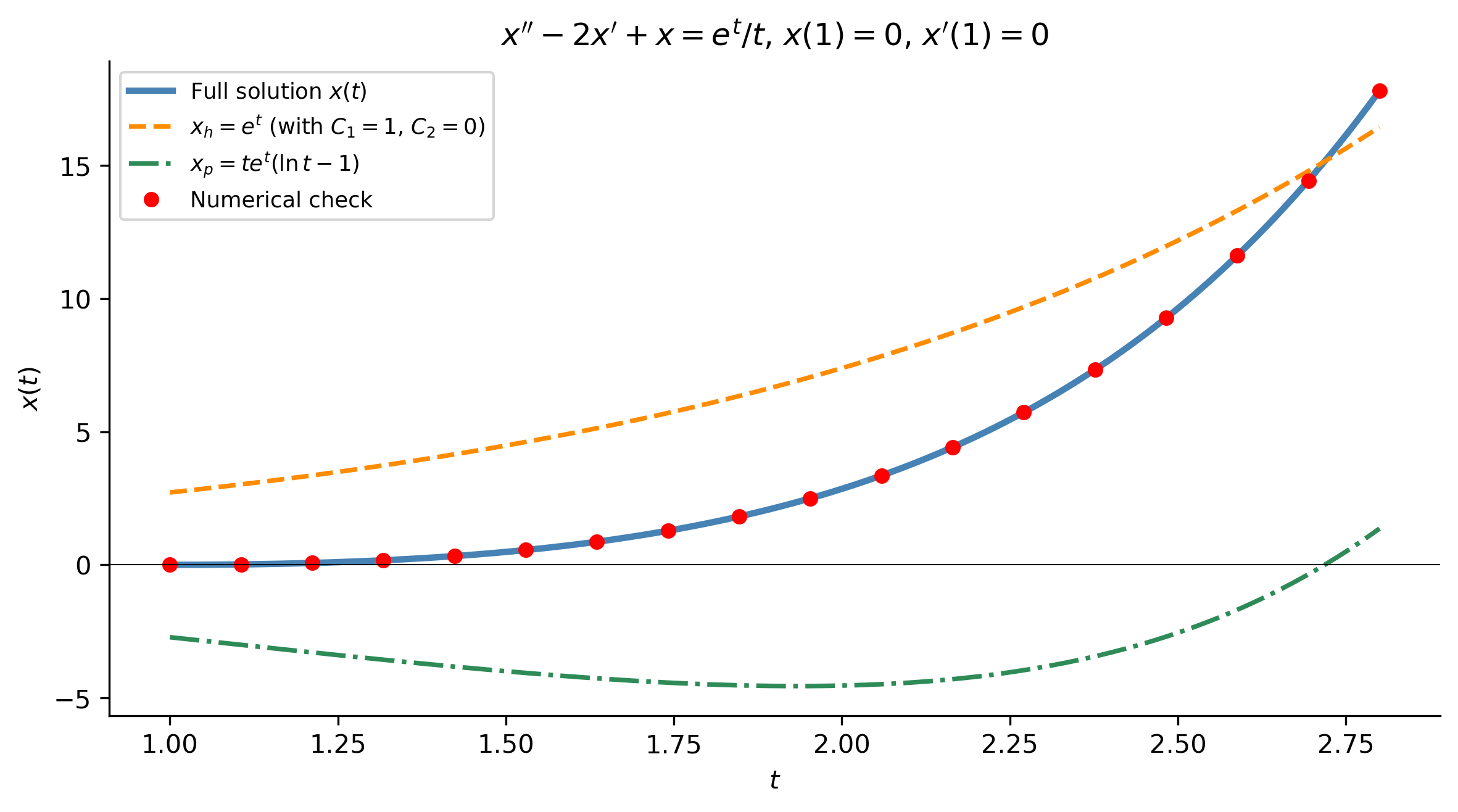
Figure 2: Example 2: \(x''-2x'+x=e^t/t\) with \(x(1)=0\), \(x'(1)=0\). The constants \(C_1=2\), \(C_2=-1\) are determined by the IVP. The particular solution \(te^t(\ln t-1)\) (green) grows rapidly for large \(t\) since it inherits the \(e^t\) factor of the homogeneous solutions. Red dots confirm the analytical formula via numerical solve.
This is a second-order linear ODE with variable coefficients — the coefficients \(t^2\) and \(-2t\) are functions of \(t\), not constants. The homogeneous part is an Euler–Cauchy equation, whose solutions are powers of \(t\).
Step 2. For the homogeneous Euler equation \(t^2 x'' - 2tx' + 2x = 0\), try \(x = t^r\). The motivation is that the Euler equation has a scaling symmetry: replacing \(t\) by \(ct\) leaves the equation’s structure unchanged, and \(t^r\) is the family of functions preserved under this scaling — just as \(e^{\lambda t}\) is preserved under differentiation for constant-coefficient equations. Substituting: \[r(r-1)t^r - 2rt^r + 2t^r = t^r[r^2 - 3r + 2] = t^r(r-1)(r-2) = 0.\] So \(r = 1\) and \(r = 2\), giving: \[x_1 = t, \qquad x_2 = t^2.\]
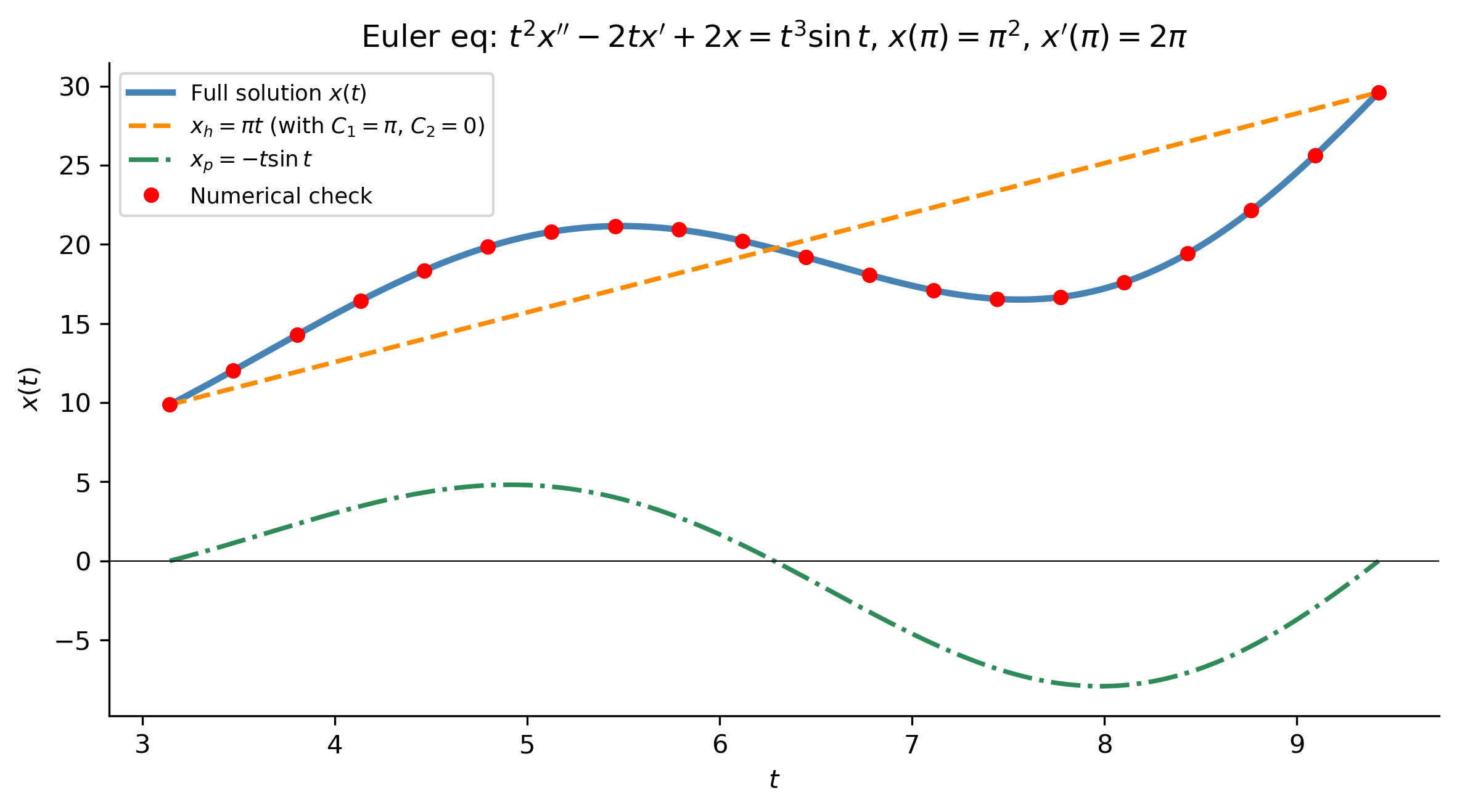
Figure 3: Example 3: Euler equation \(t^2 x''-2tx'+2x=t^3\sin t\) with \(x(\pi)=\pi^2\), \(x'(\pi)=2\pi\). The variable-coefficient homogeneous part has power-law solutions \(t\) and \(t^2\) rather than exponentials. The particular solution \(x_p=-t\sin t\) (green) oscillates with linearly growing envelope. Red dots are the numerical check.
Example 4 — \(x'' + x = \csc t\)
Another trigonometric forcing function outside the undetermined-coefficients table.
Step 1. Already in standard form; \(g(t) = \csc t\).
Step 2. Same homogeneous equation as Example 1: \[x_1 = \cos t, \qquad x_2 = \sin t, \qquad W = 1.\]
General solution:\[\boxed{x(t) = C_1\cos t + C_2\sin t - t\cos t + \sin t\ln|\sin t|.}\]
Tip
Compare Examples 1 and 4: both use \(x_1 = \cos t\), \(x_2 = \sin t\), and \(W = 1\). The only difference is the forcing — \(\sec t\) versus \(\csc t\) — yet the particular solutions are qualitatively different (\(\cos t\ln|\cos t| + t\sin t\) vs. \(-t\cos t + \sin t\ln|\sin t|\)). The method of variation of parameters is identical in both cases; only the integrals change. This illustrates how the method adapts automatically to the forcing, without any guessing or modification rule.
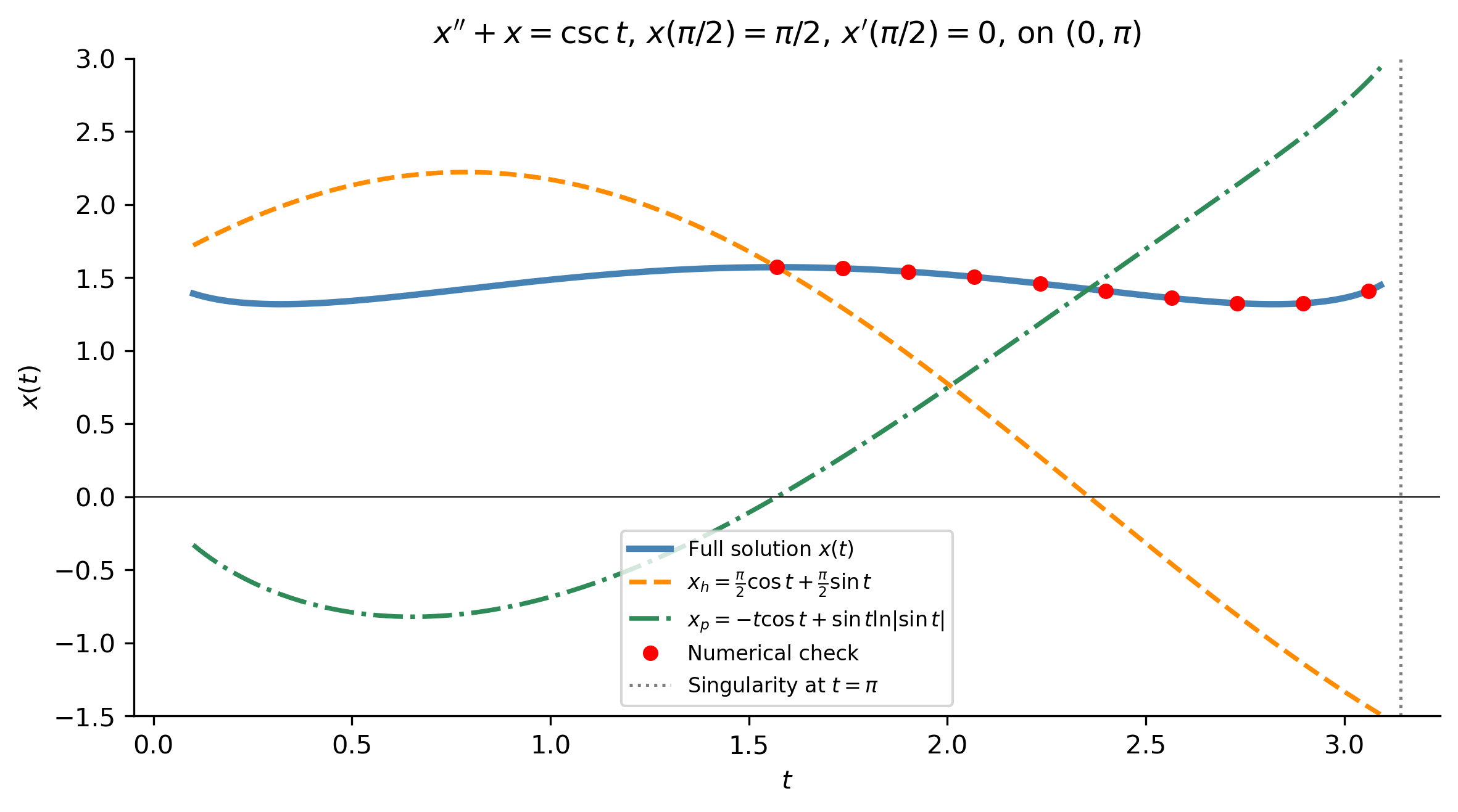
Figure 4: Example 4: \(x''+x=\csc t\), \(x(\pi/2)=\pi/2\), \(x'(\pi/2)=0\). The particular solution \(x_p=-t\cos t+\sin t\ln|\sin t|\) (green) combines the linear-growth feature \(-t\cos t\) of a near-resonant response with the logarithmic term \(\sin t\ln|\sin t|\) that vanishes at \(t=0,\pi,\ldots\) (where \(\csc t\) is singular). Red dots confirm numerically.
\(f(t)\) is a polynomial, exponential, \(\sin\), \(\cos\), or their products; and the ODE has constant coefficients
Variation of parameters
\(f(t)\) is any continuous function (\(\sec t\), \(\tan t\), \(\ln t\), \(1/t\), etc.) or the ODE has variable coefficients
Tip
Always try undetermined coefficients first when applicable — it is faster and avoids potentially difficult integrals. Switch to variation of parameters when the forcing falls outside the UC table, or when the coefficients of the ODE depend on \(t\).
Summary
Key Takeaways
Variation of parameters applies to any second-order linear ODE in standard form — constant or variable coefficients, any continuous \(g(t)\).
The side condition\(u_1'x_1+u_2'x_2=0\) is what makes the system solvable and keeps the algebra manageable.
The Wronskian\(W=x_1 x_2'-x_2 x_1'\) is the key quantity — it must be non-zero on the interval (guaranteed by linear independence of \(x_1\), \(x_2\)).
Forcing functions outside the UC table (\(\sec t\), \(\csc t\), \(1/t\), \(\ln t\), etc.) lead to non-elementary integrals — but SymPy handles them automatically.
For Euler equations, the homogeneous solutions are powers \(t^r\) rather than exponentials; variation of parameters proceeds identically once \(x_1\), \(x_2\) are found.
With the method of variation of parameters, we now have a complete toolkit for second-order linear ODEs — constant or variable coefficients, any continuous forcing. The next major step is to reframe everything in matrix language: a second-order ODE \(x'' + px' + qx = 0\) is equivalent to the first-order system \(\mathbf{y}' = A\mathbf{y}\), and the homogeneous solutions \(x_1\), \(x_2\) become columns of the fundamental matrix. The Wronskian becomes the determinant of that matrix, Abel’s identity becomes Liouville’s theorem, and variation of parameters extends naturally to systems of any size. This unification is the subject of Chapter 3 of Logan (2015).
Note
Next: Introduction to Laplace transforms — Logan §3.1.
Relevant Videos
The Wronskian:
Variation of Parameters:
References
Logan, J David. 2015. A First Course in Differential Equations, Third Edition.
TipExpand for Session Info
Show the code
import sysprint("Python version:", sys.version)print('\n'.join(f'{m.__name__}=={m.__version__}'for m inglobals().values() ifgetattr(m, '__version__', None)))