Notes 12

Linearization and Phase Plane Analysis of Nonlinear Systems

Show the code
import numpy as np
import sympy as sym
import matplotlib as mpl
import matplotlib.pyplot as plt
from scipy.integrate import solve_ivp
from IPython.display import Math, display
mpl.rcParams['figure.dpi'] = 150
mpl.rcParams['axes.spines.top'] = False
mpl.rcParams['axes.spines.right'] = False

Goals

In this section, we will:

  1. Revisit linearization for scalar autonomous equations \(x' = f(x)\) and extend the idea to two-dimensional nonlinear systems \(x' = f(x,y)\), \(y' = g(x,y)\).

  2. Define critical points (equilibria) of a nonlinear system and locate them by solving \(f(x_e, y_e) = 0\), \(g(x_e, y_e) = 0\) simultaneously.

  3. Derive the Jacobian matrix \(J(x_e, y_e)\) via Taylor expansion and identify it as the coefficient matrix of the linearized perturbation equations at the critical point.

  4. State the key result on behavior near a critical point: the nonlinear system inherits the qualitative behavior of its linearization, with the important exception of centers (purely imaginary eigenvalues).

  5. Apply the asymptotic stability criterion \(\text{tr}\,J < 0\) and \(\det J > 0\) to nonlinear systems.

  6. Use nullclines, the direction field, and the Jacobian analysis together to construct complete phase diagrams for nonlinear systems.

  7. Recognize when linearization fails (\(\det J = 0\)) and apply alternative techniques such as dividing and separating variables.

Note

This material corresponds to Section 5.1 of (Logan 2015).


Motivation: From Scalar to Planar

Linearization for a Single Equation (Review)

Recall from Chapter 1 the scalar autonomous equation \(x' = f(x)\). An equilibrium \(x_e\) satisfies \(f(x_e) = 0\). To analyze stability we set \(x(t) = x_e + u(t)\) where \(u\) is a small perturbation, and expand by Taylor’s theorem:

\[ u' = f(x_e + u) = f(x_e) + f'(x_e)\,u + \tfrac{1}{2}f''(x_e)\,u^2 + \cdots \]

Since \(f(x_e) = 0\) and higher-order terms are negligible for small \(u\), this approximates to

\[ u' = f'(x_e)\,u, \]

which has solution \(u(t) = u(0)\,e^{f'(x_e)t}\). The constant \(f'(x_e)\) is the stability indicator:

  • If \(f'(x_e) < 0\): small perturbations decay \(\implies\) \(x_e\) is asymptotically stable.
  • If \(f'(x_e) > 0\): small perturbations grow \(\implies\) \(x_e\) is unstable.
  • If \(f'(x_e) = 0\): no information; higher-order terms must be examined.

In this section we carry out precisely the same program for two-dimensional nonlinear systems.


Critical Points of Nonlinear Systems

Consider the nonlinear autonomous system

\[ x' = f(x, y), \tag{5.1} \] \[ y' = g(x, y), \tag{5.2} \]

where \(f\) and \(g\) are continuously differentiable functions. A critical point (also called an equilibrium or isolated equilibrium) is a point \(\mathbf{x}^* = (x_e, y_e)\) satisfying

\[ f(x_e, y_e) = 0 \quad \text{and} \quad g(x_e, y_e) = 0. \]

Critical points represent constant solutions \(x(t) \equiv x_e\), \(y(t) \equiv y_e\) for all time. To find them, solve these two algebraic equations simultaneously.

TipStrategy for Finding Critical Points

Factor each equation where possible. The zero-set of \(f(x,y) = 0\) defines one family of curves in the phase plane (the \(x\)-nullclines); the zero-set of \(g(x,y) = 0\) defines another family (the \(y\)-nullclines). Critical points are exactly the intersections of the \(x\)-nullclines with the \(y\)-nullclines.


Linearization at a Critical Point

The Taylor Expansion Argument

To study the behavior of the system near \((x_e, y_e)\), introduce small perturbations

\[ x(t) = x_e + u(t), \qquad y(t) = y_e + v(t). \]

Substituting into (5.1)–(5.2) and expanding in Taylor series about \((x_e, y_e)\):

\[ u' = f(x_e, y_e) + f_x(x_e, y_e)\,u + f_y(x_e, y_e)\,v + \cdots \] \[ v' = g(x_e, y_e) + g_x(x_e, y_e)\,u + g_y(x_e, y_e)\,v + \cdots \]

Since \((x_e, y_e)\) is a critical point, the first terms \(f(x_e, y_e) = g(x_e, y_e) = 0\) vanish, and for small perturbations the higher-order terms are negligible. The perturbation dynamics near the critical point are therefore governed by the linear system

\[ u' = f_x(x_e, y_e)\,u + f_y(x_e, y_e)\,v, \] \[ v' = g_x(x_e, y_e)\,u + g_y(x_e, y_e)\,v. \]


The Jacobian Matrix

In matrix form, writing \(\mathbf{z}(t) = (u(t), v(t))^T\), the linearized system is

\[ \mathbf{z}' = J\,\mathbf{z}, \tag{5.3} \]

where

ImportantDefinition: Jacobian Matrix

The Jacobian matrix of system (5.1)–(5.2) at the critical point \((x_e, y_e)\) is the matrix of first partial derivatives

\[ J(x_e, y_e) = \begin{pmatrix} f_x(x_e, y_e) & f_y(x_e, y_e) \\ g_x(x_e, y_e) & g_y(x_e, y_e) \end{pmatrix}. \tag{5.4} \]

The entries of \(J\) are constants (partial derivatives evaluated at the equilibrium). The linearized system (5.3) is a linear system with constant coefficients, exactly the type analyzed in Chapter 4.

The nature of the critical point \((0,0)\) of the linearization (5.3) is determined entirely by the eigenvalues of \(J\) — which we already know how to classify via \(\text{tr}\,J\) and \(\det J\).

NoteGeometric Interpretation

Locally, near \((x_e, y_e)\), the phase portrait of the nonlinear system (5.1)–(5.2) is a slightly distorted version of the phase portrait of the linear system \(\mathbf{z}' = J\mathbf{z}\) near the origin. The distortion arises from the nonlinear terms that were dropped to obtain the linearization.


Behavior Near a Critical Point

The relationship between the nonlinear system and its linearization is summarized in the following key results. We assume throughout that \(\det J \neq 0\) (so the critical point is isolated).

ImportantBehavior Near a Critical Point
  • Asymptotically stable. If \((0,0)\) is asymptotically stable for the linearization (5.3) — i.e., \(J\) has negative eigenvalues or complex eigenvalues with negative real part — then perturbations decay and \((x_e, y_e)\) is asymptotically stable for the nonlinear system (5.1)–(5.2). The conditions are: \[ \text{tr}\,J(x_e, y_e) < 0 \quad \text{and} \quad \det J(x_e, y_e) > 0. \tag{5.5} \]

  • Unstable. If \((0,0)\) is unstable for the linearization — i.e., \(J\) has a positive eigenvalue or complex eigenvalues with positive real part — then some or all perturbations grow and \((x_e, y_e)\) is unstable for the nonlinear system.

  • Exceptional case — center. If \((0,0)\) is a center for the linearization (purely imaginary eigenvalues of \(J\)), then \((x_e, y_e)\) may be a center or a spiral (stable or unstable) for the nonlinear system. Linearization is inconclusive in this case.

  • Borderline case — equal eigenvalues. The nonlinear system maintains its stability/instability, but the local orbital shape may change; for example, a node for the linearized system may become a spiral for the nonlinear system.

TipThe Key Practical Test (Condition 5.5)

Most of the time we only need to know whether an equilibrium is asymptotically stable or unstable. Simply compute \(\text{tr}\,J\) and \(\det J\) at the equilibrium and check: \[\text{tr}\,J < 0 \quad\text{and}\quad \det J > 0 \implies \text{asymptotically stable.}\]


Nullclines and the Phase Diagram

Nullclines are an essential tool for sketching the global phase diagram of a nonlinear system.

ImportantDefinition: Nullclines

For the system \(x' = f(x,y)\), \(y' = g(x,y)\):

  • The \(x\)-nullclines are the curves where \(f(x,y) = 0\): along these curves the vector field points straight up or down (vertical flow).
  • The \(y\)-nullclines are the curves where \(g(x,y) = 0\): along these curves the vector field points straight left or right (horizontal flow).
  • Critical points are the intersections of \(x\)-nullclines with \(y\)-nullclines, where the vector field vanishes entirely.

Procedure for Sketching Phase Diagrams

The following seven-step procedure from the text gives a systematic method for constructing the phase diagram of any nonlinear autonomous system.

  1. Find all critical points by solving \(f(x,y) = 0\) and \(g(x,y) = 0\) simultaneously. Check the type and stability of each by examining the eigenvalues of \(J\) (or equivalently, \(\text{tr}\,J\) and \(\det J\)).

  2. Draw the \(x\)- and \(y\)-nullclines. These divide the phase plane into regions.

  3. Determine the direction of the vector field in each region bounded by the nullclines. Use the sign of \(f(x,y)\) (positive \(\implies\) rightward; negative \(\implies\) leftward) and the sign of \(g(x,y)\) (positive \(\implies\) upward; negative \(\implies\) downward). Describe the combined direction geographically: NE, SE, SW, NW.

  4. Sketch representative orbits consistent with the directions found above.

  5. Find separatrix directions at saddle points and nodes by computing the eigenvectors of \(J\) at those critical points. For nonlinear systems, separatrices are curved (unlike the straight linear orbits of Chapter 4), but the eigenvectors indicate their initial directions.

  6. Divide and integrate to find orbits as curves \(y = y(x)\) when the system is simple enough to allow separation of variables.

  7. Use software to produce an accurate phase diagram with numerically computed orbits.


Example 5.1 — A System with Two Critical Points

Consider the system

\[ x' = f(x,y) = -x + xy, \tag{5.6} \] \[ y' = g(x,y) = -4y + 8xy. \tag{5.7} \]

Step 1 — Find the Critical Points

Solve \(f = 0\) and \(g = 0\) simultaneously. Factor:

\[ x(-1 + y) = 0 \implies x = 0 \quad\text{or}\quad y = 1. \] \[ 4y(-1 + 2x) = 0 \implies y = 0 \quad\text{or}\quad x = \tfrac{1}{2}. \]

  • Case \(x = 0\): substituting into \(4y(-1+2x)=0\) gives \(4y(-1)=0\), so \(y = 0\).
  • Case \(y = 1\): substituting into \(4(1)(-1+2x)=0\) gives \(x = \tfrac{1}{2}\).

The two critical points are \((0,0)\) and \(\bigl(\tfrac{1}{2}, 1\bigr)\).

Step 2 — Compute the Jacobian

\[ J(x,y) = \begin{pmatrix} f_x & f_y \\ g_x & g_y \end{pmatrix} = \begin{pmatrix} -1+y & x \\ 8y & -4+8x \end{pmatrix}. \]

At \((0,0)\):

\[ J(0,0) = \begin{pmatrix} -1 & 0 \\ 0 & -4 \end{pmatrix}, \]

which is diagonal with eigenvalues \(\lambda = -1, -4\). Since both are negative, \((0,0)\) is an asymptotically stable node (\(\text{tr}\,J = -5 < 0\), \(\det J = 4 > 0\)).

At \(\bigl(\tfrac{1}{2},1\bigr)\):

\[ J\!\left(\tfrac{1}{2},1\right) = \begin{pmatrix} 0 & \tfrac{1}{2} \\ 8 & 0 \end{pmatrix}. \]

Characteristic equation: \(\lambda^2 - 4 = 0\), so \(\lambda = \pm 2\). Opposite-sign real eigenvalues \(\implies\) \(\bigl(\tfrac{1}{2},1\bigr)\) is an unstable saddle point (\(\det J = -4 < 0\)).

Step 3 — Nullclines and Direction Field

The \(x\)-nullclines (\(f = 0\)) are the lines \(x = 0\) and \(y = 1\); the vector field is vertical along these.

The \(y\)-nullclines (\(g = 0\)) are the lines \(y = 0\) and \(x = \tfrac{1}{2}\); the vector field is horizontal along these.

At the test point \((1, -1)\) (in the 4th quadrant): \(x' = -1+(1)(-1) = -2 < 0\), \(y' = 4+8(-1) = -4 < 0\), so the direction is SW.

Show the code
def f51(x, y): return -x + x*y
def g51(x, y): return -4*y + 8*x*y

lim = 2.0
x_g, y_g = np.meshgrid(np.linspace(-lim, lim, 24), np.linspace(-lim, lim, 24))
dx = f51(x_g, y_g); dy = g51(x_g, y_g)
nrm = np.sqrt(dx**2 + dy**2 + 1e-10)

fig, ax = plt.subplots(figsize=(8, 7))
ax.quiver(x_g, y_g, dx/nrm, dy/nrm, alpha=0.3, color='gray', scale=28)

# Nullclines
ax.axvline(0,  color='steelblue', ls='--', lw=1.8, label=r"$x$-nullcline: $x=0$")
ax.axhline(1,  color='steelblue', ls='--', lw=1.8, label=r"$x$-nullcline: $y=1$")
ax.axhline(0,  color='crimson',   ls='--', lw=1.8, label=r"$y$-nullcline: $y=0$")
ax.axvline(0.5,color='crimson',   ls='--', lw=1.8, label=r"$y$-nullcline: $x=1/2$")

# Orbits
np.random.seed(7)
ics = [(1.5, 1.5), (1.5, 0.5), (1.5, -0.5), (1.5, -1.5),
       (-1.5, 1.5), (-1.5, 0.5), (-1.5, -0.5), (-1.5, -1.5),
       (0.3, 1.5), (0.8, 1.5), (-0.3, 0.5), (-0.8, 0.5),
       (0.3, -0.5), (0.8, -0.5), (0.1, 0.1), (-0.1, 0.1)]
for x0, y0 in ics:
    sol = solve_ivp(lambda t, z: [f51(z[0], z[1]), g51(z[0], z[1])],
                    (0, 6), [x0, y0], dense_output=True, max_step=0.02)
    xy = sol.y; mask = np.all(np.abs(xy) < lim*1.35, axis=0)
    ax.plot(xy[0, mask], xy[1, mask], 'k-', lw=1.0, alpha=0.55)

# Critical points
ax.plot(0, 0, 'o', color='steelblue', markersize=9, zorder=5, label='Stable node $(0,0)$')
ax.plot(0.5, 1, 's', color='crimson', markersize=9, zorder=5, label='Saddle $(1/2,1)$')

ax.set_xlim(-lim, lim); ax.set_ylim(-lim, lim)
ax.set_xlabel('$x$'); ax.set_ylabel('$y$')
ax.set_title(r"Example 5.1: $x'=-x+xy$, $y'=-4y+8xy$", fontsize=11)
ax.legend(fontsize=8, loc='lower right')
plt.tight_layout()
plt.show()
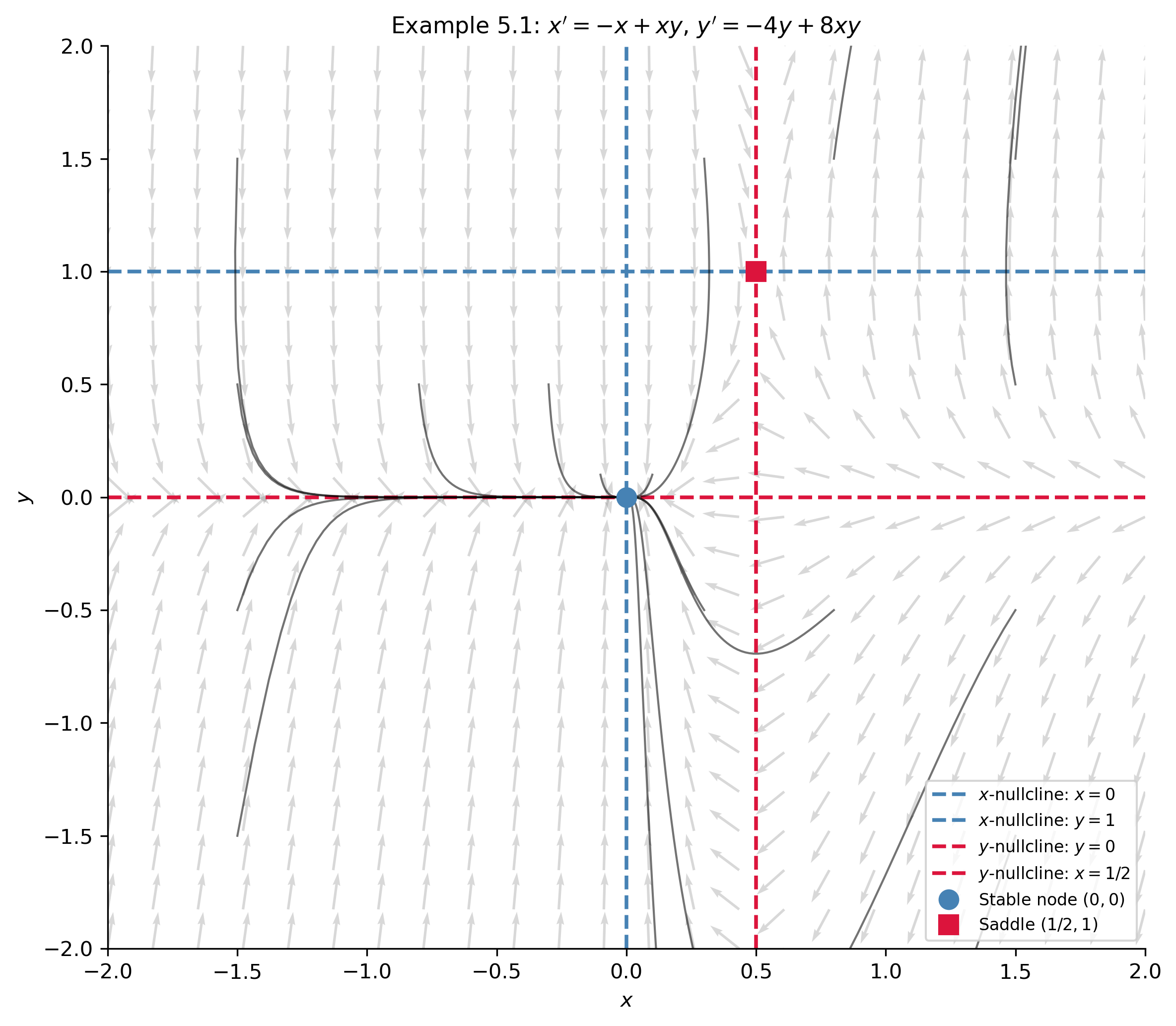
Figure 1: Phase diagram for Example 5.1: \(x'=-x+xy\), \(y'=-4y+8xy\). The \(x\)-nullclines (steelblue dashed: \(x=0\) and \(y=1\)) and \(y\)-nullclines (crimson dashed: \(y=0\) and \(x=1/2\)) divide the plane into eight regions. The origin is an asymptotically stable node (\(\lambda=-1,-4\)); the point \((1/2,1)\) is a saddle (\(\lambda=\pm 2\)). Orbits were computed using solve_ivp.

Example 5.2 — Three Critical Points

Consider the decoupled nonlinear system

\[ x' = x - x^3, \qquad y' = 2y. \]

The equilibria satisfy \(x - x^3 = x(1-x^2) = 0\) and \(2y = 0\), giving \(x = 0, \pm 1\) and \(y = 0\): three critical points at \((0,0)\), \((1,0)\), and \((-1,0)\).

The Jacobian at an arbitrary \((x,y)\) is diagonal:

\[ J(x,y) = \begin{pmatrix} 1 - 3x^2 & 0 \\ 0 & 2 \end{pmatrix}. \]

Evaluating at each critical point:

At \((0,0)\): \(J = \begin{pmatrix}1 & 0\\0 & 2\end{pmatrix}\), eigenvalues \(1\) and \(2\). Both positive \(\implies\) \((0,0)\) is an unstable node.

At \((\pm 1, 0)\): \(J = \begin{pmatrix}-2 & 0\\0 & 2\end{pmatrix}\), eigenvalues \(-2\) and \(2\). Opposite signs \(\implies\) \((\pm 1, 0)\) are both unstable saddle points.

The \(x\)-nullclines (\(x' = 0\)) are \(x = 0\), \(x = 1\), \(x = -1\) (vertical vector field); the \(y\)-nullcline (\(y' = 0\)) is \(y = 0\) (horizontal vector field). Along the \(x\)-axis: \(x' > 0\) for \(-1 < x < 1\) (rightward) and \(x' < 0\) for \(|x| > 1\) (leftward).

Show the code
def f52(x, y): return x - x**3
def g52(x, y): return 2*y

lim = 2.0
x_g, y_g = np.meshgrid(np.linspace(-lim, lim, 24), np.linspace(-lim, lim, 24))
dx = f52(x_g, y_g); dy = g52(x_g, y_g)
nrm = np.sqrt(dx**2 + dy**2 + 1e-10)

fig, ax = plt.subplots(figsize=(8, 7))
ax.quiver(x_g, y_g, dx/nrm, dy/nrm, alpha=0.3, color='gray', scale=28)

# Nullclines
for xv in [-1, 0, 1]:
    lbl = r"$x$-nullcline" if xv == -1 else None
    ax.axvline(xv, color='steelblue', ls='--', lw=1.8, label=lbl)
ax.axhline(0, color='crimson', ls='--', lw=1.8, label=r"$y$-nullcline: $y=0$")

# Orbits
ics52 = [(1.5, 0.1), (1.5, -0.1), (-1.5, 0.1), (-1.5, -0.1),
         (0.5, 0.1), (0.5, -0.1), (-0.5, 0.1), (-0.5, -0.1),
         (0.05, 1.5), (0.05, -1.5), (-0.05, 1.5), (-0.05, -1.5),
         (1.5, 1.0), (-1.5, 1.0), (1.5, -1.0), (-1.5, -1.0)]
for x0, y0 in ics52:
    sol = solve_ivp(lambda t, z: [f52(z[0], z[1]), g52(z[0], z[1])],
                    (0, 1.5), [x0, y0], dense_output=True, max_step=0.02)
    xy = sol.y; mask = np.all(np.abs(xy) < lim*1.35, axis=0)
    ax.plot(xy[0, mask], xy[1, mask], 'k-', lw=1.0, alpha=0.55)

# Critical points
ax.plot(0,  0, 'o', color='darkorange', markersize=9, zorder=5, label='Unstable node $(0,0)$')
ax.plot(1,  0, 's', color='crimson',    markersize=9, zorder=5, label='Saddle $(\\pm 1,0)$')
ax.plot(-1, 0, 's', color='crimson',    markersize=9, zorder=5)

ax.set_xlim(-lim, lim); ax.set_ylim(-lim, lim)
ax.set_xlabel('$x$'); ax.set_ylabel('$y$')
ax.set_title(r"Example 5.2: $x'=x-x^3$, $y'=2y$", fontsize=11)
ax.legend(fontsize=8, loc='lower right')
plt.tight_layout()
plt.show()
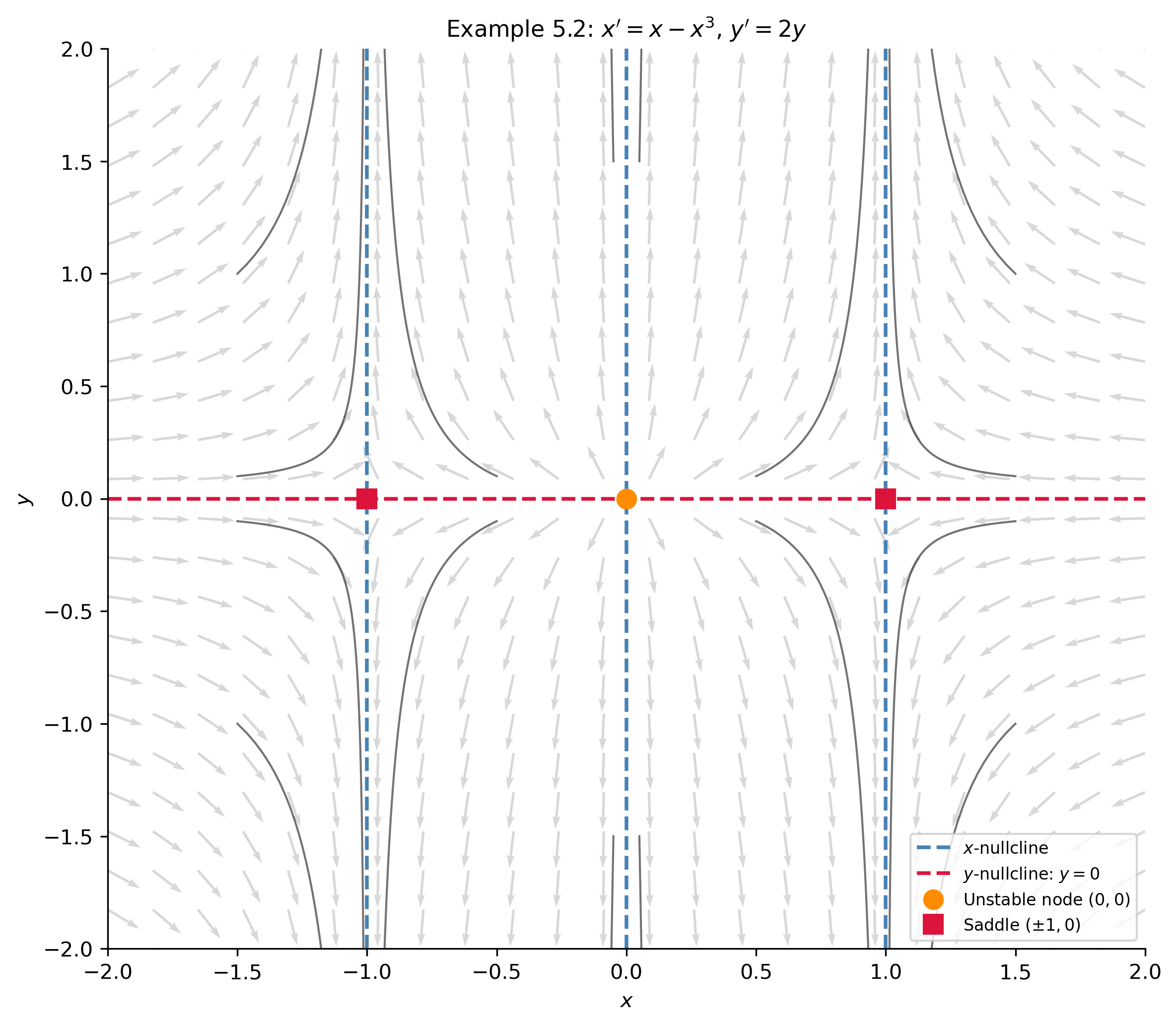
Figure 2: Phase diagram for Example 5.2: \(x'=x-x^3\), \(y'=2y\). Vertical nullclines at \(x=0,\pm 1\) (steelblue dashed) and horizontal nullcline \(y=0\) (crimson dashed). The origin is an unstable node; \((\pm 1, 0)\) are saddle points. In the upper half-plane orbits move upward; in the lower half-plane downward.

Example 5.3 — When Linearization Fails

Consider the system

\[ x' = y^2, \tag{5.8} \] \[ y' = -\tfrac{2}{3}x. \tag{5.9} \]

The only critical point is the origin \((0,0)\). The Jacobian at the origin is

\[ J(0,0) = \begin{pmatrix} 0 & 0 \\ -\tfrac{2}{3} & 0 \end{pmatrix}, \]

which has \(\det J = 0\) and both eigenvalues equal to zero. The linearization procedure does not apply because \(\det J = 0\) violates the assumption of an isolated critical point with nonzero Jacobian determinant.

Alternative: Divide and Integrate

Since both equations are known, we can divide to eliminate time:

\[ \frac{dy}{dx} = \frac{y'}{x'} = \frac{-\tfrac{2}{3}x}{y^2}, \]

and separate variables:

\[ y^2\,dy = -\tfrac{2}{3}x\,dx \implies 3y^2\,dy = -2x\,dx. \]

Integrating:

\[ y^3 = -x^2 + C, \quad\text{i.e.,}\quad y = (C - x^2)^{1/3}. \]

These are the orbits as curves in the phase plane (with the time direction requiring a separate check). Since \(x' = y^2 \ge 0\), all orbits move to the right as time increases. This example illustrates that the behavior of a nonlinear system near a degenerate critical point can differ substantially from anything in the linear classification.

Show the code
fig, ax = plt.subplots(figsize=(8, 6.5))

# Analytical orbit family
x_plot = np.linspace(-1.0, 1.0, 400)
colors_c = plt.cm.viridis(np.linspace(0.1, 0.9, 9))
for C, color in zip(np.linspace(-0.8, 0.8, 9), colors_c):
    arg = C - x_plot**2
    valid = arg > -1e-8   # cube root is real for all real arg, but avoid domain issues
    y_curve = np.cbrt(C - x_plot**2)
    ax.plot(x_plot[valid], y_curve[valid], color=color, lw=1.8, alpha=0.75)

# Numerical orbits to confirm and show direction
ics53 = [(0.0, 0.7), (0.0, -0.7), (0.0, 0.4), (0.0, -0.4),
         (-0.8, 0.0), (-0.8, 0.3), (-0.8, -0.3), (0.5, 0.6)]
for x0, y0 in ics53:
    sol = solve_ivp(lambda t, z: [z[1]**2, -2/3*z[0]],
                    (0, 3), [x0, y0], dense_output=True, max_step=0.02)
    xy = sol.y; mask = np.all(np.abs(xy) < 1.1, axis=0)
    ax.plot(xy[0, mask], xy[1, mask], 'k-', lw=1.1, alpha=0.55)
    if mask.sum() > 5:
        mid = mask.sum() // 2
        ax.annotate('', xy=(xy[0, mask][mid+2], xy[1, mask][mid+2]),
                    xytext=(xy[0, mask][mid], xy[1, mask][mid]),
                    arrowprops=dict(arrowstyle='->', color='k', lw=1.2))

# Nullclines: x-nullcline is y=0 (x'=y^2=0), y-nullcline is x=0
ax.axhline(0, color='steelblue', ls='--', lw=1.8, label=r"$x$-nullcline: $y=0$")
ax.axvline(0, color='crimson',   ls='--', lw=1.8, label=r"$y$-nullcline: $x=0$")

ax.plot(0, 0, 'ko', markersize=9, zorder=5, label=r'Critical point $(0,0)$, $\det J=0$')
ax.set_xlim(-1.0, 1.0); ax.set_ylim(-1.0, 1.0)
ax.set_xlabel('$x$'); ax.set_ylabel('$y$')
ax.set_title(r"Example 5.3: $x'=y^2$, $y'=-\frac{2}{3}x$ — degenerate critical point", fontsize=11)
ax.legend(fontsize=8, loc='upper right')
plt.tight_layout()
plt.show()
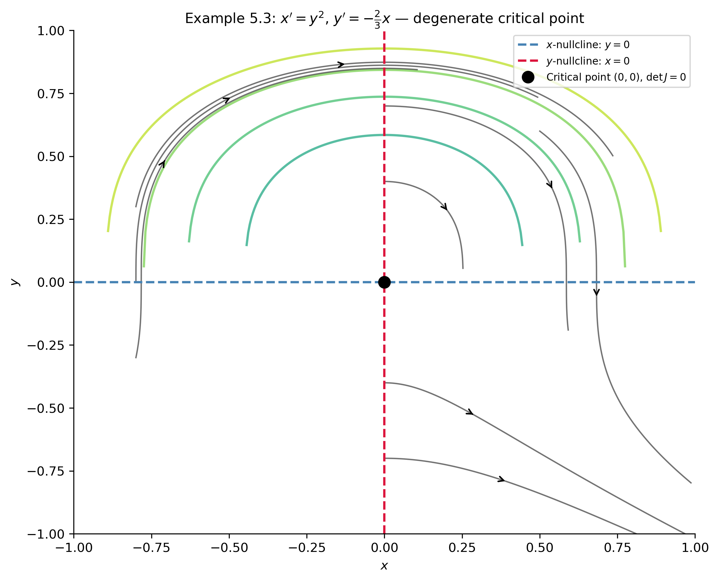
Figure 3: Phase diagram for Example 5.3: \(x'=y^2\), \(y'=-\frac{2}{3}x\). Orbits are the curves \(y=(C-x^2)^{1/3}\) for various values of \(C\) (colored curves). The critical point at the origin has \(\det J=0\), so linearization fails. Since \(x'=y^2\geq 0\), all orbits move to the right (arrows shown). Numerical solve_ivp orbits (black) confirm the analytical family.
NoteKey Lesson from Example 5.3

When \(\det J(x_e, y_e) = 0\), the standard classification (node, saddle, spiral, center) does not apply and linearization gives no information. In these cases we must use other methods: dividing the equations to find orbits directly, using conservation laws, or applying higher-order analysis. Unusual orbital behavior is common for nonlinear systems near degenerate critical points.


Summary: The Complete Analysis Workflow

The following table collects all the key formulas and results from Section 5.1.

Step What to do Key formula / test
Critical points Solve \(f=0\) and \(g=0\) simultaneously Intersections of nullclines
Jacobian Compute partial derivatives and evaluate at each equilibrium \(J = \begin{pmatrix}f_x & f_y \\ g_x & g_y\end{pmatrix}\) at \((x_e,y_e)\)
Asymp. stability Check trace and determinant \(\text{tr}\,J < 0\) and \(\det J > 0\)
Type Classify via eigenvalues of \(J\) Same table as Chapter 4
Exceptional case Purely imaginary eigenvalues Type inconclusive: may be center or spiral
Degenerate case \(\det J = 0\) Linearization fails; divide and integrate
Phase diagram Nullclines, direction field, Jacobian eigenvectors Seven-step procedure above
TipLooking Ahead

Section 5.2 applies linearization to nonlinear mechanics: Newton’s law \(mx'' = F(x, x')\) written as a system \(x' = y\), \(y' = F(x,y)/m\). The critical points correspond to equilibrium positions of the particle, and their type (center vs. spiral, stable vs. unstable) has direct physical meaning in terms of oscillatory vs. monotone behavior.


These notes are also viewable as a slide deck presentation: Open slides in full screen

Note

Next: Nonlinear Mechanics — Logan §5.2.


Relevant Videos

Linearization and the Jacobian Matrix:

Linearization Example:

Nullclines and Phase Portraits for Nonlinear Systems:

References

Logan, J David. 2015. A First Course in Differential Equations, Third Edition.
Show the code
import sys
print("Python version:", sys.version)
print('\n'.join(f'{m.__name__}=={m.__version__}' for m in globals().values() if getattr(m, '__version__', None)))
Python version: 3.14.4 | packaged by conda-forge | (main, Apr  8 2026, 02:33:53) [Clang 20.1.8 ]
numpy==2.4.3
sympy==1.14.0
matplotlib==3.10.8

Reuse

CC BY-NC-SA 4.0
