Notes 13

Applications of Nonlinear Systems

Show the code
import numpy as np
import sympy as sym
import matplotlib as mpl
import matplotlib.pyplot as plt
from scipy.integrate import solve_ivp
from IPython.display import Math, display
mpl.rcParams['figure.dpi'] = 150
mpl.rcParams['axes.spines.top'] = False
mpl.rcParams['axes.spines.right'] = False

Goals

In this section, we will:

  1. Apply the linearization and phase plane techniques from §5.1 to Lotka–Volterra predator–prey models, identifying the non-trivial equilibrium as a center for the linearization and describing the closed periodic orbits of the nonlinear system.

  2. Analyze competing species models from population ecology, classifying the four equilibria and determining which species survives depending on the relative competition strengths.

  3. Derive and study the SIR epidemic model, locating the disease-free and endemic equilibria and applying the stability criterion to find the basic reproduction number \(R_0\) that determines whether an epidemic occurs.

  4. Apply nonlinear systems analysis to chemical kinetics via the law of mass action, analyzing equilibria and the approach to chemical equilibrium.

  5. Study the nonlinear pendulum as a prototypical physics application, distinguishing the center (oscillatory) equilibria from the saddle (unstable) equilibria and computing the phase portrait including the separatrix that bounds oscillation vs. rotation.

  6. Analyze the van der Pol oscillator from nonlinear circuit theory, identifying the unstable origin and the attracting limit cycle that represents sustained oscillations.

Note

This material corresponds to Section 5.3 of (Logan 2015).


Section 5.3 — Applications of Nonlinear Systems

The methods developed in §5.1 — linearization, the Jacobian matrix, nullclines, and the phase diagram procedure — are powerful tools for qualitative analysis of nonlinear systems. In this section we apply them to classical models in population ecology, epidemiology, chemistry, and physics and engineering. In each case we:

  1. Write down the governing equations and interpret each term physically.
  2. Find all critical points by solving \(f = g = 0\).
  3. Compute \(J\) at each critical point and classify it via \(\text{tr}\,J\) and \(\det J\).
  4. Describe the phase portrait and interpret the dynamics.

Lotka–Volterra Predator–Prey Model

The Model

One of the most celebrated models in mathematical biology is the Lotka–Volterra predator–prey system, introduced independently by Alfred Lotka (1925) and Vito Volterra (1926) to explain oscillations in fish populations in the Adriatic Sea. Let \(x = x(t)\) be the prey population and \(y = y(t)\) the predator population. The model is

\[ x' = ax - bxy, \tag{5.14} \] \[ y' = -cy + dxy, \tag{5.15} \]

where all parameters \(a, b, c, d > 0\). The term \(ax\) represents the prey birth rate (exponential growth in the absence of predators); \(-bxy\) represents predation (encounters reduce prey); \(-cy\) represents the predator death rate in the absence of prey; and \(dxy\) represents predator population growth fueled by prey consumption.

Critical Points

Setting \(x' = 0\) and \(y' = 0\):

\[ x(a - by) = 0 \implies x = 0 \quad\text{or}\quad y = \frac{a}{b}. \] \[ y(-c + dx) = 0 \implies y = 0 \quad\text{or}\quad x = \frac{c}{d}. \]

The critical points are \((0, 0)\) and \(\left(\dfrac{c}{d},\, \dfrac{a}{b}\right)\).

Jacobian Analysis

The general Jacobian is

\[ J(x,y) = \begin{pmatrix} a - by & -bx \\ dy & -c + dx \end{pmatrix}. \]

At \((0,0)\): \(J = \begin{pmatrix}a & 0 \\ 0 & -c\end{pmatrix}\), eigenvalues \(a > 0\) and \(-c < 0\). Opposite signs \(\implies\) \((0,0)\) is an unstable saddle point. (If both populations vanish the system is at an unstable equilibrium — a slight perturbation drives population growth.)

At \(\left(\dfrac{c}{d},\dfrac{a}{b}\right)\): substituting,

\[ J\!\left(\frac{c}{d},\frac{a}{b}\right) = \begin{pmatrix} 0 & -bc/d \\ da/b & 0 \end{pmatrix}. \]

The characteristic equation is \(\lambda^2 + ac = 0\), giving purely imaginary eigenvalues \(\lambda = \pm i\sqrt{ac}\).

ImportantThe Non-Trivial Equilibrium is a Center (Linearization)

For the linearized system, \(\left(\dfrac{c}{d},\dfrac{a}{b}\right)\) is a center — orbits are closed ellipses around it. Because this is the exceptional case (purely imaginary eigenvalues), linearization cannot confirm whether the nonlinear system has a center or a spiral.

For the Lotka–Volterra system, one can show by finding a conserved quantity (first integral) that the orbits of the nonlinear system are also closed. Dividing (5.15) by (5.14) and separating variables yields

\[ \frac{-c + dx}{x}\,dx + \frac{a - by}{y}\,dy = 0, \]

which integrates to

\[ H(x,y) = dx - c\ln x + by - a\ln y = \text{constant}. \]

The level curves of \(H(x,y)\) are the orbits — they are closed curves surrounding the non-trivial equilibrium, confirming that the populations oscillate periodically in the nonlinear system as well.

NoteEcological Interpretation

The periodic orbits of the Lotka–Volterra model describe the classic boom–bust cycle: when prey are abundant, predator populations grow; growing predator numbers reduce prey; declining prey then cause predator decline; with fewer predators, prey recover — and the cycle repeats. Volterra used this model to explain why Italian fishermen observed an increase in the relative proportion of sharks (predators) during WWI, when fishing (which removes both species) was greatly reduced.

Show the code
a, b, c, d = 0.6, 0.5, 0.3, 0.4
xe, ye = c/d, a/b   # non-trivial equilibrium

def f_lv(x, y): return a*x - b*x*y
def g_lv(x, y): return -c*y + d*x*y

fig, axes = plt.subplots(1, 2, figsize=(11, 5))

# Phase portrait
lim_x, lim_y = 3.0, 3.0
x_g, y_g = np.meshgrid(np.linspace(0.02, lim_x, 22),
                        np.linspace(0.02, lim_y, 22))
dx = f_lv(x_g, y_g); dy = g_lv(x_g, y_g)
nrm = np.sqrt(dx**2 + dy**2 + 1e-10)
axes[0].quiver(x_g, y_g, dx/nrm, dy/nrm, alpha=0.25, color='gray', scale=28)

# Nullclines
x_nc = np.linspace(0.01, lim_x, 300)
axes[0].axvline(xe, color='crimson', ls='--', lw=1.8,
                label=rf"$y$-nullcline: $x={xe:.2f}$")
axes[0].axhline(ye, color='steelblue', ls='--', lw=1.8,
                label=rf"$x$-nullcline: $y={ye:.2f}$")
axes[0].axhline(0,  color='gray', ls='--', lw=0.8)
axes[0].axvline(0,  color='gray', ls='--', lw=0.8)

# Closed orbits
colors_orb = plt.cm.viridis(np.linspace(0.15, 0.85, 5))
for r_frac, color in zip([0.15, 0.35, 0.55, 0.75, 0.95], colors_orb):
    x0 = xe + r_frac * xe
    sol = solve_ivp(lambda t, z: [f_lv(z[0], z[1]), g_lv(z[0], z[1])],
                    (0, 60), [x0, ye], dense_output=True,
                    max_step=0.05, rtol=1e-8, atol=1e-10)
    xy = sol.y
    mask = (xy[0] > 0) & (xy[1] > 0) & (xy[0] < lim_x) & (xy[1] < lim_y)
    axes[0].plot(xy[0, mask], xy[1, mask], color=color, lw=1.5)

axes[0].plot(xe, ye, 'o', color='steelblue', markersize=9, zorder=6,
             label=f'Equil. $({xe:.2f},{ye:.2f})$ — center')
axes[0].plot(0, 0, 's', color='crimson', markersize=8, zorder=6,
             label='Origin — saddle')
axes[0].set_xlim(0, lim_x); axes[0].set_ylim(0, lim_y)
axes[0].set_xlabel('$x$ (prey)'); axes[0].set_ylabel('$y$ (predator)')
axes[0].set_title('Phase portrait')
axes[0].legend(fontsize=8)

# Time series
x0_ts, y0_ts = xe + 0.5*xe, ye
sol_ts = solve_ivp(lambda t, z: [f_lv(z[0], z[1]), g_lv(z[0], z[1])],
                   (0, 40), [x0_ts, y0_ts], dense_output=True,
                   max_step=0.05, rtol=1e-8, atol=1e-10)
t_plot = np.linspace(0, 40, 800)
axes[1].plot(t_plot, sol_ts.sol(t_plot)[0], color='steelblue', lw=2.5,
             label='$x(t)$ prey')
axes[1].plot(t_plot, sol_ts.sol(t_plot)[1], color='crimson', lw=2.5,
             label='$y(t)$ predator')
axes[1].axhline(xe, color='steelblue', ls=':', lw=1, alpha=0.7)
axes[1].axhline(ye, color='crimson',   ls=':', lw=1, alpha=0.7)
axes[1].set_xlabel('$t$'); axes[1].set_ylabel('Population')
axes[1].set_title('Time series')
axes[1].legend(fontsize=9)

plt.suptitle(f'Lotka–Volterra: $a={a}$, $b={b}$, $c={c}$, $d={d}$', fontsize=12)
plt.tight_layout()
plt.show()
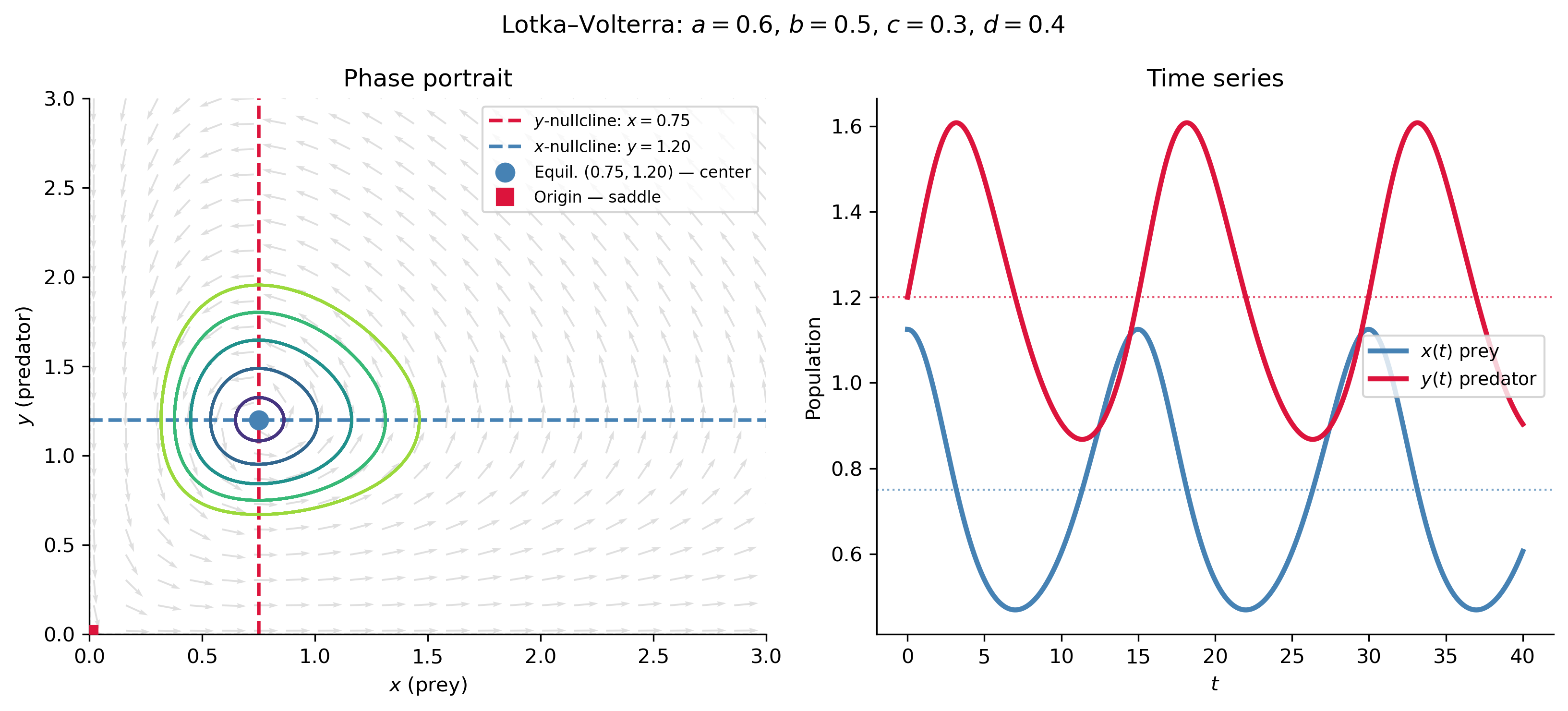
Figure 1: Lotka–Volterra predator–prey model with \(a=0.6\), \(b=0.5\), \(c=0.3\), \(d=0.4\). Left: phase portrait showing closed orbits encircling the non-trivial equilibrium \((c/d, a/b) = (0.75, 1.2)\) (blue dot). The origin is an unstable saddle. Right: time series for a representative orbit showing the characteristic out-of-phase oscillations between prey \(x(t)\) (steelblue) and predator \(y(t)\) (crimson).

Competing Species Model

The Model

When two species compete for the same resource, neither benefits from the other’s presence. Let \(x\) and \(y\) denote the two species populations. A classical model is

\[ x' = x(a_1 - b_1 x - c_1 y), \tag{5.16} \] \[ y' = y(a_2 - b_2 y - c_2 x), \tag{5.17} \]

where \(a_i, b_i, c_i > 0\). Each species follows logistic growth (\(a_i - b_i N_i\)) in isolation; the additional terms \(-c_1 y\) and \(-c_2 x\) represent the competitive reduction in growth rate due to the other species.

Critical Points

The equilibria are found by solving \(x' = g = 0\):

  • \((0,0)\) — both extinct.
  • \((a_1/b_1, 0)\) — species \(x\) alone at its carrying capacity.
  • \((0, a_2/b_2)\) — species \(y\) alone at its carrying capacity.
  • Interior equilibrium \((x^*, y^*)\) — coexistence, found by solving the linear system \(b_1 x + c_1 y = a_1\) and \(c_2 x + b_2 y = a_2\).

The stability of the interior equilibrium and the axis equilibria determines the outcome of competition. For specific parameters, this can be analyzed via the Jacobian at each point:

\[ J(x,y) = \begin{pmatrix} a_1 - 2b_1 x - c_1 y & -c_1 x \\ -c_2 y & a_2 - 2b_2 y - c_2 x \end{pmatrix}. \]

The key ecological outcomes depend on whether \(c_1/b_1\) and \(c_2/b_2\) are large or small relative to \(a_1/b_1\) and \(a_2/b_2\):

  • One species wins — the interior equilibrium is a saddle; one of the axis equilibria is stable.
  • Coexistence — the interior equilibrium is a stable node or spiral; both species survive.
Show the code
fig, axes = plt.subplots(1, 2, figsize=(11, 5))

def competing(a1, b1, c1, a2, b2, c2):
    def f_(x, y): return x*(a1 - b1*x - c1*y)
    def g_(x, y): return y*(a2 - b2*y - c2*x)
    return f_, g_

cases = [
    dict(a1=1, b1=1, c1=0.3, a2=1, b2=1, c2=0.5,
         title="Weak competition — Coexistence\n($c_1=0.3$, $c_2=0.5$)"),
    dict(a1=1, b1=1, c1=1.4, a2=1, b2=1, c2=1.2,
         title="Strong competition — Exclusion\n($c_1=1.4$, $c_2=1.2$)"),
]

for ax, case in zip(axes, cases):
    a1,b1,c1,a2,b2,c2 = (case[k] for k in ('a1','b1','c1','a2','b2','c2'))
    f_, g_ = competing(a1,b1,c1,a2,b2,c2)

    lim = 1.6
    x_g, y_g = np.meshgrid(np.linspace(0, lim, 22), np.linspace(0, lim, 22))
    dx = f_(x_g, y_g); dy = g_(x_g, y_g)
    nrm = np.sqrt(dx**2 + dy**2 + 1e-10)
    ax.quiver(x_g, y_g, dx/nrm, dy/nrm, alpha=0.25, color='gray', scale=28)

    # Nullclines
    x_nc = np.linspace(0, lim, 300)
    ax.plot(x_nc, (a1 - b1*x_nc)/c1, 'steelblue', ls='--', lw=1.8,
            label=r"$x'=0$")
    ax.plot(x_nc, (a2 - c2*x_nc)/b2, 'crimson', ls='--', lw=1.8,
            label=r"$y'=0$")

    # Orbits
    np.random.seed(42)
    for _ in range(14):
        x0 = np.random.uniform(0.05, 1.4)
        y0 = np.random.uniform(0.05, 1.4)
        sol = solve_ivp(lambda t, z: [f_(z[0],z[1]), g_(z[0],z[1])],
                        (0, 20), [x0, y0], dense_output=True, max_step=0.05)
        xy = sol.y
        mask = (xy[0]>=0) & (xy[1]>=0) & (xy[0]<=lim) & (xy[1]<=lim)
        ax.plot(xy[0,mask], xy[1,mask], 'k-', lw=0.9, alpha=0.5)

    ax.plot(0, 0, 'ks', markersize=7, zorder=5)
    ax.plot(a1/b1, 0, 'o', color='steelblue', markersize=8, zorder=5)
    ax.plot(0, a2/b2, 'o', color='crimson', markersize=8, zorder=5)

    # Interior equilibrium
    denom = b1*b2 - c1*c2
    if abs(denom) > 1e-6:
        xs = (a1*b2 - c1*a2)/denom
        ys = (a2*b1 - c2*a1)/denom
        if xs > 0 and ys > 0:
            color_int = 'seagreen' if c1*c2 < b1*b2 else 'darkorange'
            ax.plot(xs, ys, '*', color=color_int, markersize=12, zorder=6,
                    label=f'Interior $({xs:.2f},{ys:.2f})$')

    ax.set_xlim(0, lim); ax.set_ylim(0, lim)
    ax.set_xlabel('$x$'); ax.set_ylabel('$y$')
    ax.set_title(case['title'], fontsize=10)
    ax.legend(fontsize=8)

plt.suptitle("Competing Species Model", fontsize=12)
plt.tight_layout()
plt.show()
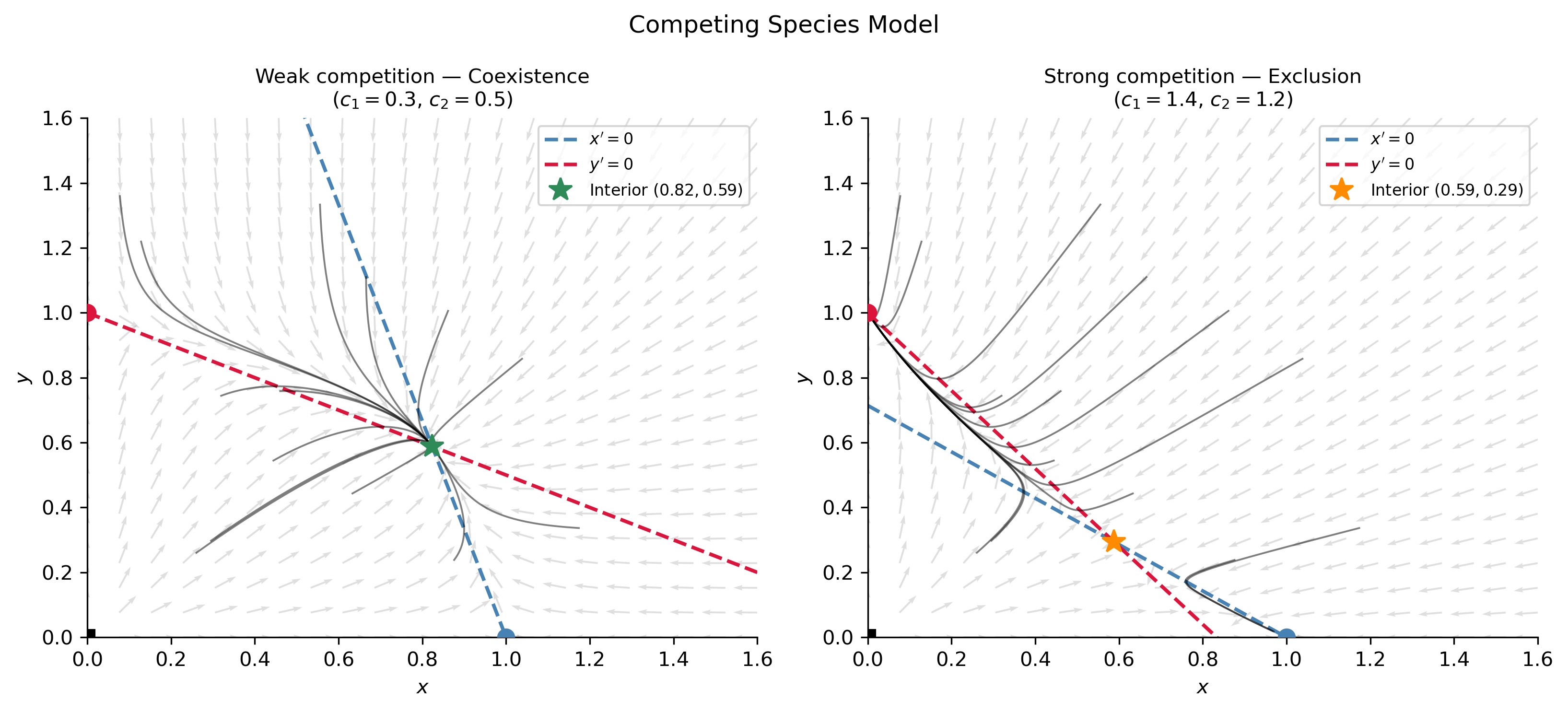
Figure 2: Competing species phase portraits with \(a_1=a_2=1\), \(b_1=b_2=1\). Left: weak competition (\(c_1=0.3\), \(c_2=0.5\)) — coexistence; the interior equilibrium is a stable node and both species survive. Right: strong competition (\(c_1=1.4\), \(c_2=1.2\)) — competitive exclusion; the interior equilibrium is a saddle, and the outcome depends on initial conditions (species \(x\) wins above the separatrix, species \(y\) wins below).

The SIR Epidemic Model

The Model

A fundamental model in mathematical epidemiology is the SIR model (Kermack–McKendrick, 1927). The population is divided into three compartments:

  • \(S = S(t)\): Susceptible individuals who can catch the disease.
  • \(I = I(t)\): Infected individuals who can transmit the disease.
  • \(R = R(t)\): Removed individuals who have recovered (and are immune) or died.

The model equations are

\[ S' = -\beta SI, \tag{5.18} \] \[ I' = \beta SI - \gamma I, \tag{5.19} \] \[ R' = \gamma I, \tag{5.20} \]

where \(\beta > 0\) is the transmission rate (rate at which susceptibles are infected per contact) and \(\gamma > 0\) is the recovery rate (rate at which infected individuals are removed). Since \(S + I + R = N\) (constant total population), the system reduces to the two-dimensional \((S, I)\) system (5.18)–(5.19).

The Basic Reproduction Number \(R_0\)

The key question in epidemiology is: will a small introduction of infected individuals into a fully susceptible population cause an epidemic? From equation (5.19):

\[ I' = I(\beta S - \gamma). \]

At the start of an outbreak with \(S \approx N\):

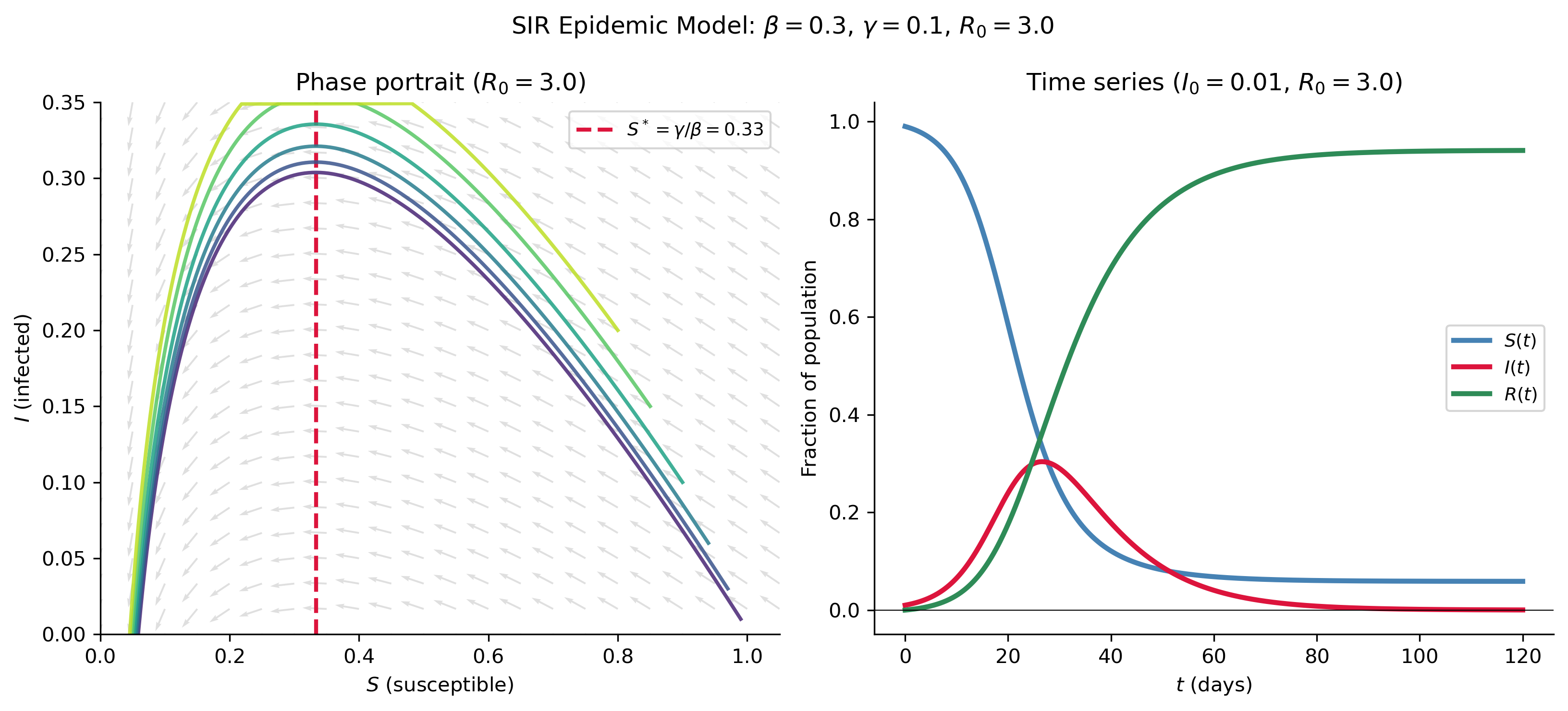
  • If \(\beta N / \gamma > 1\): \(I' > 0\) and the infection spreads — epidemic occurs.
  • If \(\beta N / \gamma < 1\): \(I' < 0\) and the infection dies out — no epidemic.
ImportantThe Basic Reproduction Number

\[R_0 = \frac{\beta N}{\gamma}\] is the basic reproduction number — the average number of secondary infections produced by one infected individual in a fully susceptible population.

  • \(R_0 > 1\): epidemic occurs.
  • \(R_0 < 1\): infection dies out.

Critical Points and Linearization

The critical points of (5.18)–(5.19) satisfy \(\beta SI = 0\) and \(I(\beta S - \gamma) = 0\). This gives the line of equilibria \(I = 0\) (any \(S \ge 0\)) — the disease-free states. The biologically relevant analysis concerns the stability of the disease-free equilibrium \((S^*, 0)\) for \(S^* > 0\).

The Jacobian is

\[ J(S,I) = \begin{pmatrix} -\beta I & -\beta S \\ \beta I & \beta S - \gamma \end{pmatrix}. \]

At a disease-free point \((S^*, 0)\):

\[ J(S^*, 0) = \begin{pmatrix} 0 & -\beta S^* \\ 0 & \beta S^* - \gamma \end{pmatrix}, \]

with eigenvalues \(\lambda_1 = 0\) and \(\lambda_2 = \beta S^* - \gamma\). The disease-free equilibrium is stable (infection decreases) if and only if \(\lambda_2 < 0\), i.e., \(\beta S^* < \gamma\), i.e., \(R_0 = \beta S^*/\gamma < 1\).

Show the code
beta, gamma_sir = 0.3, 0.1
N = 1.0
R0 = beta * N / gamma_sir
print(f"R_0 = beta*N/gamma = {R0:.2f}")

def f_sir(S, I): return -beta * S * I
def g_sir(S, I): return beta * S * I - gamma_sir * I

fig, axes = plt.subplots(1, 2, figsize=(11, 5))

# Phase portrait in (S, I) plane
lim_S, lim_I = 1.05, 0.35
S_g, I_g = np.meshgrid(np.linspace(0, lim_S, 22), np.linspace(0, lim_I, 22))
dS = f_sir(S_g, I_g); dI = g_sir(S_g, I_g)
nrm = np.sqrt(dS**2 + dI**2 + 1e-10)
axes[0].quiver(S_g, I_g, dS/nrm, dI/nrm, alpha=0.25, color='gray', scale=28)

S_thresh = gamma_sir / beta
axes[0].axvline(S_thresh, color='crimson', ls='--', lw=2.0,
                label=rf"$S^*=\gamma/\beta={S_thresh:.2f}$")

colors_ic = plt.cm.viridis(np.linspace(0.1, 0.9, 6))
for I0, color in zip([0.01, 0.03, 0.06, 0.10, 0.15, 0.20], colors_ic):
    S0 = N - I0
    sol = solve_ivp(lambda t, z: [f_sir(z[0],z[1]), g_sir(z[0],z[1])],
                    (0, 200), [S0, I0], dense_output=True,
                    max_step=0.1, rtol=1e-8, atol=1e-10)
    Si = sol.y
    mask = (Si[0]>=0) & (Si[1]>=0) & (Si[0]<=lim_S) & (Si[1]<=lim_I)
    axes[0].plot(Si[0,mask], Si[1,mask], color=color, lw=1.8, alpha=0.85)

axes[0].set_xlim(0, lim_S); axes[0].set_ylim(0, lim_I)
axes[0].set_xlabel('$S$ (susceptible)'); axes[0].set_ylabel('$I$ (infected)')
axes[0].set_title(f'Phase portrait ($R_0={R0:.1f}$)')
axes[0].legend(fontsize=9)

# Time series
I0_ts = 0.01; S0_ts = N - I0_ts; R0_ts = 0.0
sol_ts = solve_ivp(
    lambda t, z: [f_sir(z[0],z[1]), g_sir(z[0],z[1]), gamma_sir*z[1]],
    (0, 120), [S0_ts, I0_ts, R0_ts], dense_output=True, max_step=0.1)
t_plot = np.linspace(0, 120, 600)
vals = sol_ts.sol(t_plot)
axes[1].plot(t_plot, vals[0], color='steelblue', lw=2.5, label='$S(t)$')
axes[1].plot(t_plot, vals[1], color='crimson',   lw=2.5, label='$I(t)$')
axes[1].plot(t_plot, vals[2], color='seagreen',  lw=2.5, label='$R(t)$')
axes[1].axhline(0, color='k', lw=0.5)
axes[1].set_xlabel('$t$ (days)'); axes[1].set_ylabel('Fraction of population')
axes[1].set_title(f'Time series ($I_0={I0_ts}$, $R_0={R0:.1f}$)')
axes[1].legend(fontsize=9)

plt.suptitle(rf'SIR Epidemic Model: $\beta={beta}$, $\gamma={gamma_sir}$, $R_0={R0:.1f}$',
             fontsize=12)
plt.tight_layout()
plt.show()
R_0 = beta*N/gamma = 3.00
Figure 3: SIR epidemic model. Left: \((S,I)\) phase portrait with \(\beta=0.3\), \(\gamma=0.1\), \(N=1\) (so \(R_0=3>1\)). Orbits start at \(S\approx 1\) with a small initial infected fraction and sweep through an epidemic arc before settling on the \(S\)-axis (disease-free). The threshold \(S^*=\gamma/\beta=1/3\) is shown dashed. Right: time series for one orbit showing the classic epidemic curve — \(I(t)\) rises to a peak then falls as \(S\) is depleted.

Chemical Kinetics — Law of Mass Action

The Model

Many chemical reactions can be modeled as nonlinear autonomous systems using the law of mass action: the rate of a reaction is proportional to the product of the concentrations of the reacting species. Consider the reversible reaction

\[ A + B \;\underset{k_{-}}{\overset{k_{+}}{\rightleftharpoons}}\; C, \]

where \([A]\), \([B]\), and \([C]\) denote concentrations and \(k_+\), \(k_-\) are the forward and reverse rate constants. Let \(x = [A]\), \(y = [B]\), \(z = [C]\). By conservation of mass the concentrations satisfy \(x(t) + z(t) = x_0\) (constant) and \(y(t) + z(t) = y_0\) (constant), reducing the system to a single ODE in \(z\):

\[ z' = k_+(x_0 - z)(y_0 - z) - k_- z. \]

As a two-dimensional illustration, consider a system of two consecutive reactions:

\[ A \xrightarrow{k_1} B \xrightarrow{k_2} C. \]

Let \(x = [A]\) and \(y = [B]\). By mass action:

\[ x' = -k_1 x, \tag{5.21} \] \[ y' = k_1 x - k_2 y. \tag{5.22} \]

The only equilibrium is \((0,0)\) (all \(A\) converts to \(B\), which then converts to \(C\)). The Jacobian \(J = \begin{pmatrix}-k_1 & 0 \\ k_1 & -k_2\end{pmatrix}\) has eigenvalues \(-k_1\) and \(-k_2\) (both negative), so \((0,0)\) is an asymptotically stable node — all concentrations eventually reach chemical equilibrium.

Show the code
k1, k2 = 0.5, 0.2

def f_ck(x, y): return -k1 * x
def g_ck(x, y): return k1*x - k2*y

fig, axes = plt.subplots(1, 2, figsize=(11, 5))

lim = 1.1
x_g, y_g = np.meshgrid(np.linspace(0, lim, 22), np.linspace(0, lim, 22))
dx = f_ck(x_g, y_g); dy = g_ck(x_g, y_g)
nrm = np.sqrt(dx**2 + dy**2 + 1e-10)
axes[0].quiver(x_g, y_g, dx/nrm, dy/nrm, alpha=0.25, color='gray', scale=28)

colors_ck = plt.cm.plasma(np.linspace(0.1, 0.85, 6))
for x0, y0, color in zip([1.0, 0.8, 0.6, 0.4, 0.2, 0.0],
                          [0.0, 0.2, 0.2, 0.3, 0.4, 0.8], colors_ck):
    sol = solve_ivp(lambda t, z: [f_ck(z[0],z[1]), g_ck(z[0],z[1])],
                    (0, 20), [x0, y0], dense_output=True, max_step=0.1)
    xy = sol.y
    mask = (xy[0]>=0) & (xy[1]>=0) & (xy[0]<=lim) & (xy[1]<=lim)
    axes[0].plot(xy[0,mask], xy[1,mask], color=color, lw=1.8)

axes[0].plot(0, 0, 'o', color='steelblue', markersize=9, zorder=5,
             label='Stable node $(0,0)$')
axes[0].set_xlim(0, lim); axes[0].set_ylim(0, lim)
axes[0].set_xlabel('$x=[A]$'); axes[0].set_ylabel('$y=[B]$')
axes[0].set_title(r'Phase portrait ($A\to B\to C$)')
axes[0].legend(fontsize=9)

# Time series
t_plot = np.linspace(0, 20, 400)
x_t = np.exp(-k1 * t_plot)
y_t = (k1/(k2-k1)) * (np.exp(-k1*t_plot) - np.exp(-k2*t_plot))
z_t = 1 - x_t - y_t
axes[1].plot(t_plot, x_t, color='steelblue', lw=2.5, label='$[A](t)$')
axes[1].plot(t_plot, y_t, color='crimson',   lw=2.5, label='$[B](t)$')
axes[1].plot(t_plot, z_t, color='seagreen',  lw=2.5, ls='--', label='$[C](t)=1-x-y$')
axes[1].axhline(0, color='k', lw=0.5)
axes[1].set_xlabel('$t$'); axes[1].set_ylabel('Concentration')
axes[1].set_title(f'Time series ($k_1={k1}$, $k_2={k2}$)')
axes[1].legend(fontsize=9)

plt.suptitle('Chemical Kinetics: $A \\to B \\to C$', fontsize=12)
plt.tight_layout()
plt.show()
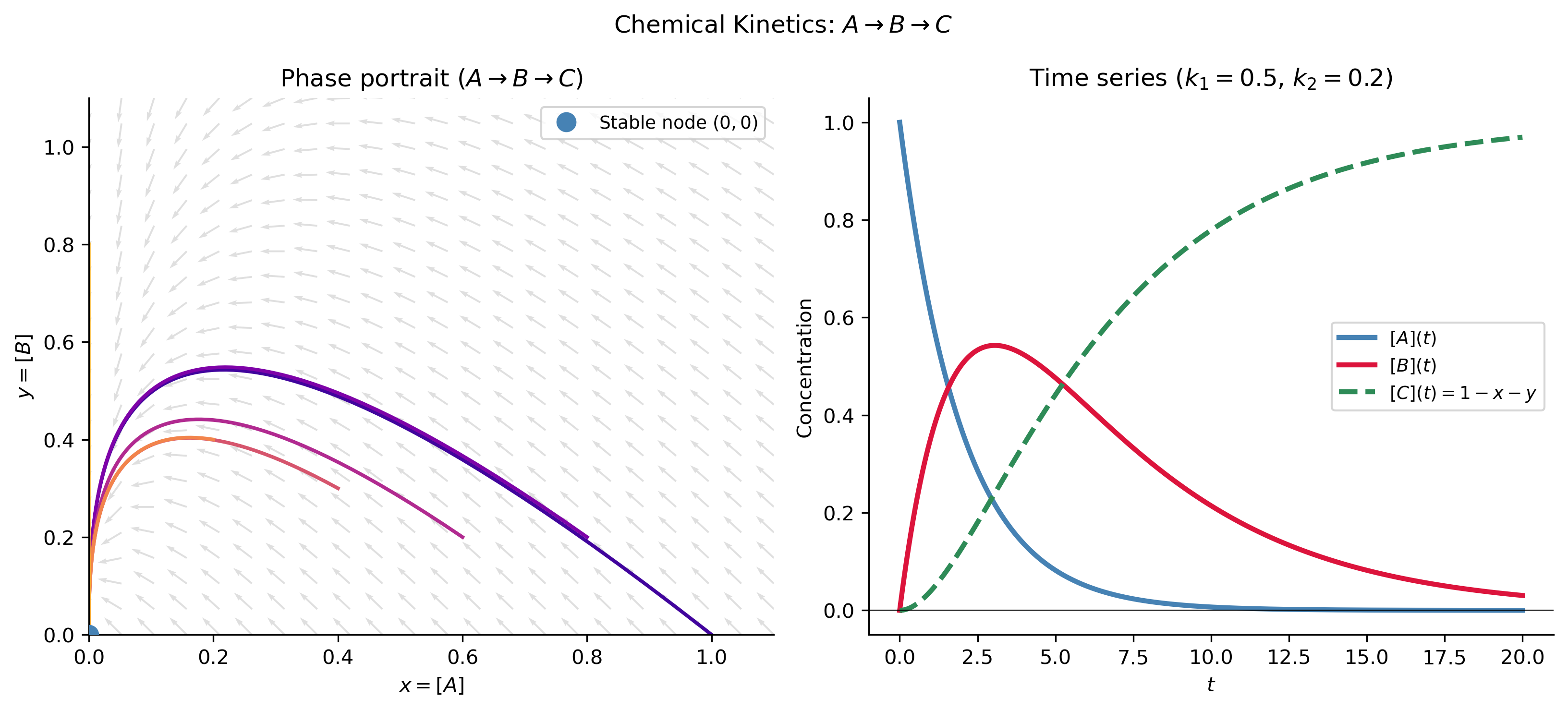
Figure 4: Consecutive reactions \(A\to B\to C\) with \(k_1=0.5\), \(k_2=0.2\). Left: \((x,y)\) phase portrait — all orbits approach the origin (stable node) as all material converts to \(C\). Right: time series starting at \([A]_0=1\), \([B]_0=0\) showing \([A]\) decays exponentially, \([B]\) rises then falls (the classic intermediate peak), and \([C]=1-x-y\) (dashed) approaches 1.

Physics Application — The Nonlinear Pendulum

The Model

The motion of a simple pendulum of length \(L\) and mass \(m\) (no damping) is governed by

\[ m L\,\theta'' = -mg\sin\theta, \]

or, with \(\omega_0^2 = g/L\),

\[ \theta'' + \omega_0^2 \sin\theta = 0. \]

Setting \(x = \theta\) (angle) and \(y = \theta'\) (angular velocity), this becomes the system

\[ x' = y, \tag{5.23} \] \[ y' = -\omega_0^2 \sin x. \tag{5.24} \]

Critical Points

Equilibria: \(y = 0\) and \(\sin x = 0\), giving \(x = n\pi\) for integer \(n\). There are two physically distinct equilibria:

  • \((0, 0)\), \((2\pi, 0)\), \(\ldots\) — pendulum hanging straight down (stable rest position).
  • \((\pi, 0)\), \((3\pi, 0)\), \(\ldots\) — pendulum pointing straight up (unstable inverted position).

Jacobian Analysis

\[ J(x,y) = \begin{pmatrix} 0 & 1 \\ -\omega_0^2\cos x & 0 \end{pmatrix}. \]

At \((0,0)\): \(J = \begin{pmatrix}0 & 1 \\ -\omega_0^2 & 0\end{pmatrix}\), characteristic equation \(\lambda^2 + \omega_0^2 = 0\), eigenvalues \(\lambda = \pm i\omega_0\). The linearization gives a center — the exceptional case. For the nonlinear pendulum, one can show using the conserved energy \(H = \tfrac{1}{2}y^2 - \omega_0^2\cos x\) that the critical point is indeed a true center with closed periodic orbits (small oscillations are approximately simple harmonic motion).

At \((\pi, 0)\): \(J = \begin{pmatrix}0 & 1 \\ \omega_0^2 & 0\end{pmatrix}\), eigenvalues \(\lambda = \pm\omega_0\). Opposite-sign real eigenvalues \(\implies\) unstable saddle point (the inverted pendulum is unstable).

Energy and the Separatrix

The system (5.23)–(5.24) is conservative with energy

\[ H(x,y) = \tfrac{1}{2}y^2 - \omega_0^2\cos x = \text{constant}. \]

Orbits lie on level curves of \(H\):

  • \(H < \omega_0^2\): closed orbits (oscillation — pendulum swings back and forth).
  • \(H = \omega_0^2\): the separatrix — the orbit passing through the saddle point \((\pi, 0)\). This is the boundary between oscillation and full rotation.
  • \(H > \omega_0^2\): open orbits (rotation — pendulum swings all the way over the top).
Show the code
omega0 = 1.0

def f_pend(x, y): return y
def g_pend(x, y): return -omega0**2 * np.sin(x)
def H_pend(x, y): return 0.5*y**2 - omega0**2 * np.cos(x)

fig, ax = plt.subplots(figsize=(10, 6))

x_g = np.linspace(-3.5*np.pi, 3.5*np.pi, 300)
y_g = np.linspace(-3.0, 3.0, 300)
X, Y = np.meshgrid(x_g, y_g)
H_vals = H_pend(X, Y)

# Filled contours for energy level
contour_f = ax.contourf(X, Y, H_vals, levels=40, cmap='RdYlBu_r', alpha=0.35)

# Level curves
levels_osc = np.linspace(-omega0**2 + 0.02, omega0**2 - 0.05, 6)
levels_rot = [omega0**2 + 0.4, omega0**2 + 1.2, omega0**2 + 2.5]
ax.contour(X, Y, H_vals, levels=levels_osc,
           colors='steelblue', linewidths=1.5, alpha=0.85)
ax.contour(X, Y, H_vals, levels=levels_rot,
           colors='seagreen', linewidths=1.5, alpha=0.85)

# Separatrix
ax.contour(X, Y, H_vals, levels=[omega0**2],
           colors='black', linewidths=2.5)

# Critical points
for n in range(-3, 4):
    xe_p = 2*n*np.pi
    ax.plot(xe_p, 0, 'o', color='steelblue', markersize=9, zorder=6)
for n in range(-2, 3):
    xe_p = (2*n+1)*np.pi
    ax.plot(xe_p, 0, 's', color='crimson', markersize=9, zorder=6)

# Legend proxies
ax.plot([], [], 'o', color='steelblue', markersize=9,
        label='Center (pendulum down — oscillation)')
ax.plot([], [], 's', color='crimson', markersize=9,
        label='Saddle (pendulum up — unstable)')
ax.plot([], [], 'k-', lw=2.5, label='Separatrix ($H=\\omega_0^2$)')
ax.plot([], [], color='steelblue', lw=1.5,
        label='Oscillating orbits ($H<\\omega_0^2$)')
ax.plot([], [], color='seagreen', lw=1.5,
        label='Rotating orbits ($H>\\omega_0^2$)')

ax.set_xlim(-3.5*np.pi, 3.5*np.pi)
ax.set_ylim(-3.0, 3.0)
ax.set_xlabel(r'$x = \theta$ (angle, radians)')
ax.set_ylabel(r"$y = \theta'$ (angular velocity)")
ax.set_title(r"Nonlinear Pendulum: $x'=y$, $y'=-\omega_0^2\sin x$ ($\omega_0=1$)", fontsize=11)
ax.set_xticks([-2*np.pi, -np.pi, 0, np.pi, 2*np.pi])
ax.set_xticklabels([r'$-2\pi$', r'$-\pi$', '$0$', r'$\pi$', r'$2\pi$'])
ax.legend(fontsize=8, loc='upper right')
plt.tight_layout()
plt.show()
Figure 5: Nonlinear pendulum phase portrait (\(\omega_0=1\)). Centers at \(x=0,\pm 2\pi,\ldots\) (steelblue, stable oscillation) and saddle points at \(x=\pm\pi,\ldots\) (crimson, unstable inverted position). The thick black curves are the separatrices connecting the saddle points, bounding oscillatory (closed) orbits from rotational (open) orbits.

Engineering Application — The van der Pol Oscillator

The Model

The van der Pol oscillator arises in the study of nonlinear electronic circuits and was introduced by Balthasar van der Pol (1926) to model oscillations in vacuum-tube circuits. The equation is

\[ \mu'' - \varepsilon(1 - \mu^2)\mu' + \mu = 0, \qquad \varepsilon > 0, \]

where \(\mu\) is a dimensionless voltage and \(\varepsilon\) controls the nonlinearity. Setting \(x = \mu\) and \(y = \mu'\), this becomes the system

\[ x' = y, \tag{5.25} \] \[ y' = \varepsilon(1 - x^2)y - x. \tag{5.26} \]

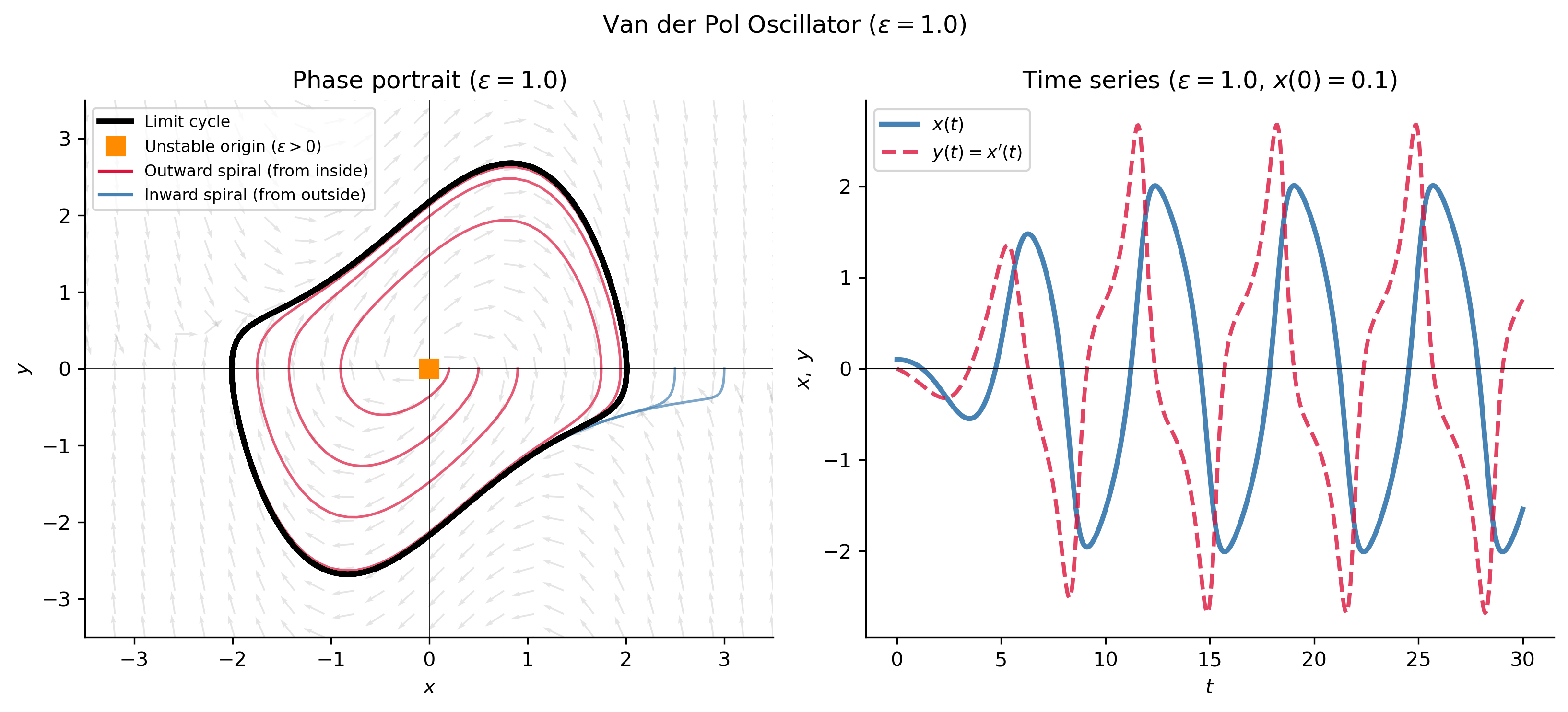
The term \(\varepsilon(1 - x^2)y\) acts as a nonlinear damping: for \(|x| < 1\) it provides negative damping (energy is added to the system); for \(|x| > 1\) it provides positive damping (energy is removed). This self-regulating mechanism produces a stable limit cycle — a periodic orbit that nearby trajectories approach asymptotically regardless of initial conditions.

Critical Point Analysis

The only critical point is the origin \((0,0)\). The Jacobian is

\[ J(x,y) = \begin{pmatrix} 0 & 1 \\ -1 - 2\varepsilon xy & \varepsilon(1-x^2) \end{pmatrix}. \]

At \((0,0)\): \(J = \begin{pmatrix}0 & 1 \\ -1 & \varepsilon\end{pmatrix}\), with \(\text{tr}\,J = \varepsilon > 0\) and \(\det J = 1 > 0\). Since the trace is positive, \((0,0)\) is an unstable spiral (or unstable node for large \(\varepsilon\)). Orbits starting near the origin spiral outward toward the limit cycle; orbits starting far from the origin are pulled inward toward the limit cycle.

NoteLimit Cycles

The van der Pol oscillator is a canonical example of a system with a stable limit cycle — an isolated closed orbit that attracts all nearby trajectories. Limit cycles are a purely nonlinear phenomenon; they cannot occur in linear systems. They represent self-sustained oscillations that are independent of initial conditions.

Show the code
eps = 1.0

def f_vdp(x, y): return y
def g_vdp(x, y): return eps*(1 - x**2)*y - x

fig, axes = plt.subplots(1, 2, figsize=(11, 5))

lim = 3.5
x_g, y_g = np.meshgrid(np.linspace(-lim, lim, 24), np.linspace(-lim, lim, 24))
dx = f_vdp(x_g, y_g); dy = g_vdp(x_g, y_g)
nrm = np.sqrt(dx**2 + dy**2 + 1e-10)
axes[0].quiver(x_g, y_g, dx/nrm, dy/nrm, alpha=0.2, color='gray', scale=30)

# Orbits spiraling out from near origin
for r in [0.2, 0.5, 0.9]:
    sol = solve_ivp(lambda t, z: [f_vdp(z[0],z[1]), g_vdp(z[0],z[1])],
                    (0, 30), [r, 0.0], dense_output=True, max_step=0.05)
    xy = sol.y; mask = np.all(np.abs(xy) < lim+0.5, axis=0)
    axes[0].plot(xy[0,mask], xy[1,mask], color='crimson', lw=1.3, alpha=0.7)

# Orbits spiraling in from outside
for r in [3.0, 2.5]:
    sol = solve_ivp(lambda t, z: [f_vdp(z[0],z[1]), g_vdp(z[0],z[1])],
                    (0, 20), [r, 0.0], dense_output=True, max_step=0.05)
    xy = sol.y; mask = np.all(np.abs(xy) < lim+0.5, axis=0)
    axes[0].plot(xy[0,mask], xy[1,mask], color='steelblue', lw=1.3, alpha=0.7)

# Limit cycle (long-time behavior)
sol_lc = solve_ivp(lambda t, z: [f_vdp(z[0],z[1]), g_vdp(z[0],z[1])],
                   (0, 100), [0.5, 0.0], dense_output=True, max_step=0.02)
xy_lc = sol_lc.y
# Take last two periods approximately
mask_lc = sol_lc.t > 80
axes[0].plot(xy_lc[0, mask_lc], xy_lc[1, mask_lc], 'k-', lw=2.8,
             label='Limit cycle', zorder=5)

axes[0].plot(0, 0, 's', color='darkorange', markersize=9, zorder=6,
             label='Unstable origin ($\\varepsilon>0$)')
axes[0].plot([], [], color='crimson', lw=1.5, label='Outward spiral (from inside)')
axes[0].plot([], [], color='steelblue', lw=1.5, label='Inward spiral (from outside)')
axes[0].set_xlim(-lim, lim); axes[0].set_ylim(-lim, lim)
axes[0].set_xlabel('$x$'); axes[0].set_ylabel('$y$')
axes[0].set_title(f'Phase portrait ($\\varepsilon={eps}$)')
axes[0].legend(fontsize=8)
axes[0].axhline(0, color='k', lw=0.4); axes[0].axvline(0, color='k', lw=0.4)

# Time series
t_ts = np.linspace(0, 30, 600)
sol_ts = solve_ivp(lambda t, z: [f_vdp(z[0],z[1]), g_vdp(z[0],z[1])],
                   (0, 30), [0.1, 0.0], dense_output=True, max_step=0.05)
axes[1].plot(t_ts, sol_ts.sol(t_ts)[0], color='steelblue', lw=2.5, label='$x(t)$')
axes[1].plot(t_ts, sol_ts.sol(t_ts)[1], color='crimson', lw=2.0, ls='--',
             label="$y(t) = x'(t)$", alpha=0.8)
axes[1].axhline(0, color='k', lw=0.5)
axes[1].set_xlabel('$t$'); axes[1].set_ylabel('$x,\\ y$')
axes[1].set_title(f'Time series ($\\varepsilon={eps}$, $x(0)=0.1$)')
axes[1].legend(fontsize=9)

plt.suptitle(f'Van der Pol Oscillator ($\\varepsilon={eps}$)', fontsize=12)
plt.tight_layout()
plt.show()
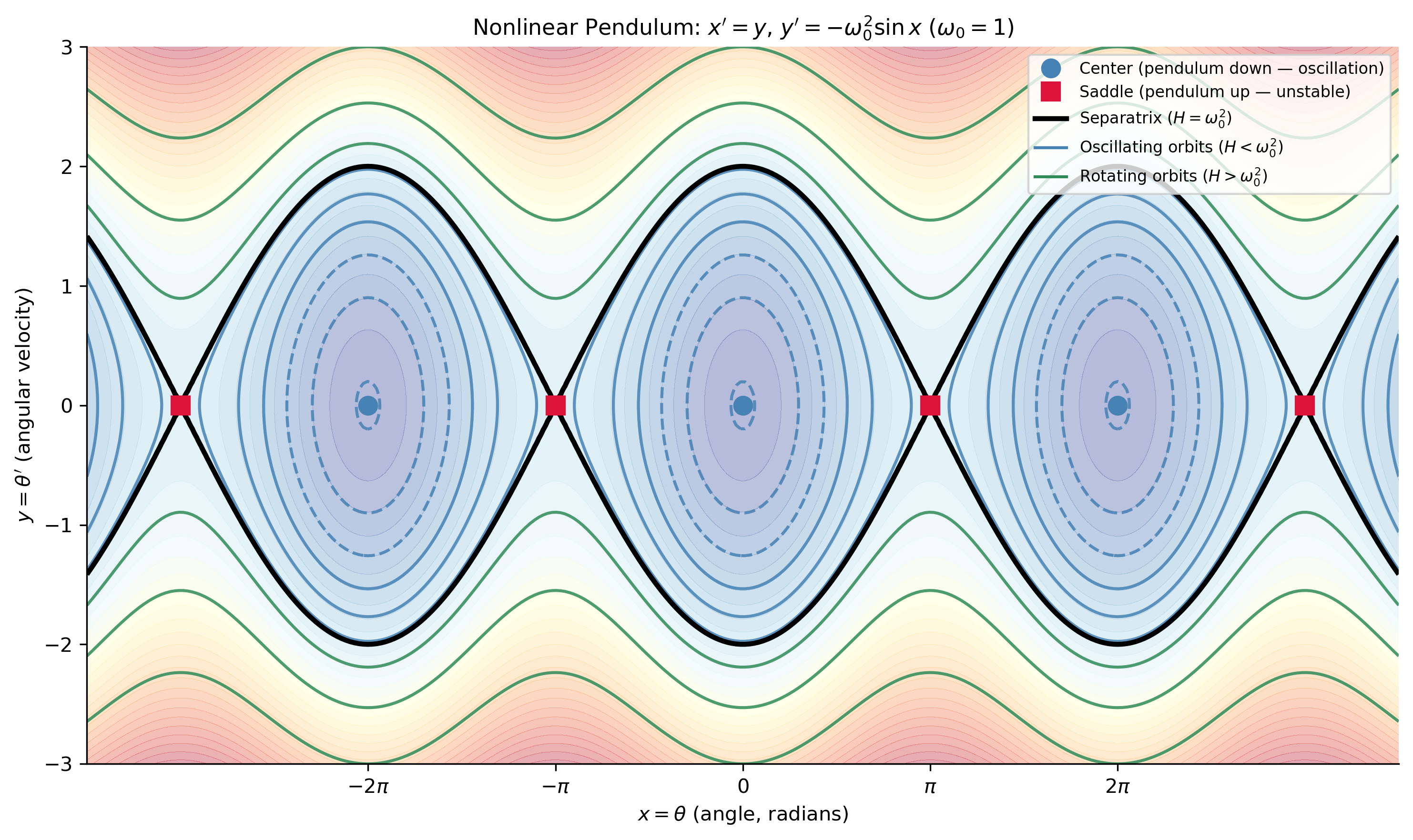
Figure 6: Van der Pol oscillator with \(\varepsilon=1\). Left: phase portrait — orbits starting near the unstable origin spiral outward (crimson) and orbits starting far from the origin spiral inward (steelblue), both converging to the same attracting limit cycle (thick black). Right: time series showing the characteristic relaxation oscillation waveform that develops from a small initial condition.

Summary

The following table collects the key models and their critical point structures from this section.

Model Equations Non-trivial equil. Type Significance
Lotka–Volterra \(x'=ax-bxy\), \(y'=-cy+dxy\) \((c/d,\,a/b)\) Center Periodic prey–predator cycles
Competing species \(x'=x(a_1-b_1x-c_1y)\), \(y'=y(a_2-b_2y-c_2x)\) \((x^*,y^*)\) Node or saddle Coexistence or exclusion
SIR epidemic \(S'=-\beta SI\), \(I'=\beta SI-\gamma I\) \(I=0\) line Stable/unstable Epidemic iff \(R_0=\beta N/\gamma>1\)
Chemical kinetics \(x'=-k_1x\), \(y'=k_1x-k_2y\) \((0,0)\) Stable node Concentrations \(\to\) equilibrium
Nonlinear pendulum \(x'=y\), \(y'=-\omega_0^2\sin x\) \((n\pi,0)\) Center / saddle Oscillation vs. rotation; separatrix
Van der Pol \(x'=y\), \(y'=\varepsilon(1-x^2)y-x\) \((0,0)\) Unstable Attracting limit cycle
TipLooking Ahead

The van der Pol oscillator is an example of a system with a limit cycle — a closed orbit that is isolated and attracting. The existence and stability of limit cycles in general planar systems is addressed by the Poincaré–Bendixson theorem and related results. Chapter 5 of Logan touches further on applications in nonlinear mechanics (§5.2) and closes with additional biological models.


These notes are also viewable as a slide deck presentation: Open slides in full screen

Note

Next: Numerical methods — Logan §6.2.


Relevant Videos

Predator–Prey and Lotka–Volterra:

The SIR Epidemic Model:

The Nonlinear Pendulum and Limit Cycles Part 1:

The Nonlinear Pendulum and Limit Cycles Part 2:

References

Logan, J David. 2015. A First Course in Differential Equations, Third Edition.
Show the code
import sys
print("Python version:", sys.version)
print('\n'.join(f'{m.__name__}=={m.__version__}' for m in globals().values() if getattr(m, '__version__', None)))
Python version: 3.14.4 | packaged by conda-forge | (main, Apr  8 2026, 02:33:53) [Clang 20.1.8 ]
numpy==2.4.3
sympy==1.14.0
matplotlib==3.10.8

Reuse

CC BY-NC-SA 4.0