Notes 10

The Eigenvalue Problem and Solving Linear Systems

Show the code
import numpy as np
import sympy as sym
import matplotlib as mpl
import matplotlib.pyplot as plt
from scipy.integrate import solve_ivp
from IPython.display import Math, display
mpl.rcParams['figure.dpi'] = 150
mpl.rcParams['axes.spines.top'] = False
mpl.rcParams['axes.spines.right'] = False

Goals

In this section, we will:

  1. Motivate the eigenvalue ansatz \(\mathbf{x} = \mathbf{v}e^{\lambda t}\) by observing that exponential solutions cancel cleanly in the system \(\mathbf{x}' = A\mathbf{x}\).

  2. Define eigenvalues, eigenvectors, and eigenpairs of a \(2\times 2\) matrix \(A\), and connect each eigenpair to a solution of \(\mathbf{x}' = A\mathbf{x}\).

  3. Solve the algebraic eigenvalue problem via the characteristic equation \(\lambda^2 - (\text{tr}\,A)\lambda + \det A = 0\) and the system \((A - \lambda I)\mathbf{v} = \mathbf{0}\).

  4. Classify and solve linear systems for the three cases of eigenvalues: real and unequal, complex conjugates, and real and equal (including the deficient case).

  5. Interpret each case geometrically through the phase plane, identifying saddle points, stable and unstable nodes, spiral points, and centers.

  6. Demonstrate the use of SymPy and solve_ivp to compute eigenpairs, write general solutions, and plot phase portraits.

Note

This material corresponds to Sections 4.3 and 4.4 of (Logan 2015).


Section 4.3 — The Eigenvalue Problem

Motivation: Exponential Solutions

We wish to solve the two-dimensional linear system

\[ \mathbf{x}' = A\mathbf{x}, \tag{4.26} \]

where \(A\) is a constant \(2\times 2\) matrix and \(\mathbf{x}(t) = (x(t),\, y(t))^T\). From our experience with scalar constant-coefficient ODEs, a solution \(x(t)\), \(y(t)\) and its derivatives must have the same form if all terms are to cancel when substituted into the equation. Exponential functions satisfy this criterion. We therefore attempt a solution of the form

\[ \mathbf{x} = \mathbf{v}e^{\lambda t}, \tag{4.27} \]

where \(\lambda\) is a constant scalar and \(\mathbf{v}\) is a nonzero constant vector, both to be determined. Substituting \(\mathbf{x} = \mathbf{v}e^{\lambda t}\) and \(\mathbf{x}' = \lambda \mathbf{v}e^{\lambda t}\) into (4.26) gives

\[ \lambda \mathbf{v}e^{\lambda t} = A(\mathbf{v}e^{\lambda t}), \]

and since \(e^{\lambda t} \neq 0\) we may cancel it to obtain the purely algebraic condition

\[ A\mathbf{v} = \lambda\mathbf{v}. \tag{4.28} \]

Therefore, if some \(\lambda\) and \(\mathbf{v}\) can be found satisfying (4.28), then \(\mathbf{x}(t) = \mathbf{v}e^{\lambda t}\) is a solution of (4.26). We have reduced a differential equations problem to an algebraic one.


Eigenvalues, Eigenvectors, and Eigenpairs

ImportantRemark 4.26 — Eigenvalue Problem

A nonzero constant vector \(\mathbf{v}\) is an eigenvector of \(A\) if \(A\mathbf{v} = \lambda\mathbf{v}\) for some scalar \(\lambda\). The scalar \(\lambda\) is called an eigenvalue of \(A\). The pair \(\lambda,\,\mathbf{v}\) is called an eigenpair. Every eigenpair of \(A\) gives a solution \(\mathbf{x}(t) = \mathbf{v}e^{\lambda t}\) of \(\mathbf{x}' = A\mathbf{x}\).

Geometrically, the eigenvalue problem (4.28) says: the matrix \(A\) represents a linear transformation acting on vectors; an eigenvector is a special vector that \(A\) transforms to a scalar multiple of itself — that multiple being the eigenvalue \(\lambda\).


Solving the Eigenvalue Problem

We rewrite \(A\mathbf{v} = \lambda\mathbf{v}\) as a homogeneous linear system:

\[ (A - \lambda I)\mathbf{v} = \mathbf{0}. \tag{4.29} \]

This system has nontrivial solutions if and only if the determinant of the coefficient matrix is zero:

\[ \det(A - \lambda I) = 0. \tag{4.30} \]

Written out explicitly for \(A = \begin{pmatrix} a & b \\ c & d \end{pmatrix}\), equation (4.30) becomes

\[ \det\begin{pmatrix} a - \lambda & b \\ c & d - \lambda \end{pmatrix} = (a-\lambda)(d-\lambda) - cb = 0, \]

or equivalently,

\[ \lambda^2 - (a+d)\lambda + (ad - bc) = 0. \tag{4.31} \]

This is most elegantly written as

\[ \lambda^2 - (\text{tr}\,A)\lambda + \det A = 0, \tag{4.32} \]

where \(\text{tr}\,A = a + d\) is the trace of \(A\), the sum of its diagonal elements. Equation (4.32) is called the characteristic equation of \(A\). It is a quadratic in \(\lambda\) whose roots — found by factoring or the quadratic formula — are the two eigenvalues of \(A\). The eigenvalues may be real and unequal, real and equal, or complex conjugates.

ImportantAlgorithm: Solving the Eigenvalue Problem \(A\mathbf{v} = \lambda\mathbf{v}\)
  1. Find eigenvalues. Solve the characteristic equation \(\det(A - \lambda I) = 0\), equivalently \[\lambda^2 - (\text{tr}\,A)\lambda + \det A = 0.\]

  2. Find eigenvectors. For each eigenvalue \(\lambda\), substitute into the homogeneous system \[(A - \lambda I)\mathbf{v} = \mathbf{0}\] and solve for \(\mathbf{v}\). Only one of the two (dependent) equations needs to be used.

Two important facts hold before proceeding to examples:

  1. Any constant multiple of an eigenvector is again an eigenvector for the same eigenvalue, since \(A(c\mathbf{v}) = cA\mathbf{v} = c(\lambda\mathbf{v}) = \lambda(c\mathbf{v})\). Thus an eigenvector is unique only up to a scalar multiple; we choose a convenient representative.

  2. If the eigenvalues are unequal, \(\lambda_1 \neq \lambda_2\), then the corresponding eigenvectors \(\mathbf{v}_1\) and \(\mathbf{v}_2\) are independent. (This is proved by contradiction — assuming \(\mathbf{v}_2 = c\mathbf{v}_1\) and applying \(A\) leads to \(\mathbf{0} = c(\lambda_1 - \lambda_2)\mathbf{v}_1\), a contradiction since all three factors are nonzero.)


Example 4.27 — Real Unequal Eigenvalues

Consider the matrix

\[ A = \begin{pmatrix} 1 & 1 \\ 4 & 1 \end{pmatrix}. \]

Characteristic equation: \(\det(A - \lambda I) = 0\) gives

\[ (1 - \lambda)^2 - 4 = \lambda^2 - 2\lambda - 3 = (\lambda + 1)(\lambda - 3) = 0. \]

Thus \(\lambda_1 = -1\) and \(\lambda_2 = 3\). Note: \(\text{tr}\,A = 2\) and \(\det A = -3\), confirming \(\lambda^2 - 2\lambda - 3 = 0\).

Eigenvectors. For \(\lambda_1 = -1\): the system \((A + I)\mathbf{v} = \mathbf{0}\) becomes

\[ \begin{pmatrix} 2 & 1 \\ 4 & 2 \end{pmatrix}\begin{pmatrix} v_1 \\ v_2 \end{pmatrix} = \begin{pmatrix} 0 \\ 0 \end{pmatrix}. \]

Both equations reduce to \(2v_1 + v_2 = 0\), so \(v_2 = -2v_1\). Taking \(v_1 = 1\) gives \(\mathbf{v}_1 = (1,\,-2)^T\).

For \(\lambda_2 = 3\): the system \((A - 3I)\mathbf{v} = \mathbf{0}\) becomes

\[ \begin{pmatrix} -2 & 1 \\ 4 & -2 \end{pmatrix}\begin{pmatrix} v_1 \\ v_2 \end{pmatrix} = \begin{pmatrix} 0 \\ 0 \end{pmatrix}. \]

Taking \(-2v_1 + v_2 = 0\), so \(v_2 = 2v_1\). With \(v_1 = 1\) we get \(\mathbf{v}_2 = (1,\,2)^T\).

The eigenpairs are therefore

\[ \lambda_1 = -1,\quad \mathbf{v}_1 = \begin{pmatrix}1\\-2\end{pmatrix} \qquad\text{and}\qquad \lambda_2 = 3,\quad \mathbf{v}_2 = \begin{pmatrix}1\\2\end{pmatrix}. \qquad\square \]

Show the code
s = sym.Symbol('lam')
A427 = sym.Matrix([[1, 1], [4, 1]])
char_poly = A427.charpoly(s)
print("Characteristic polynomial:", char_poly.as_expr())
print("Eigenvalues:", sym.solve(char_poly.as_expr(), s))
print("\nEigenvectors (SymPy):")
for val, mult, vecs in A427.eigenvects():
    for v in vecs:
        display(Math(rf"\lambda = {val},\quad \mathbf{{v}} = {sym.latex(v)}"))
Characteristic polynomial: lam**2 - 2*lam - 3
Eigenvalues: [-1, 3]

Eigenvectors (SymPy):

\(\displaystyle \lambda = -1,\quad \mathbf{v} = \left[\begin{matrix}- \frac{1}{2}\\1\end{matrix}\right]\)

(a) SymPy verification of the eigenvalues and eigenvectors for Example 4.27. The characteristic polynomial, eigenvalues, and eigenvectors all match the hand calculations.

\(\displaystyle \lambda = 3,\quad \mathbf{v} = \left[\begin{matrix}\frac{1}{2}\\1\end{matrix}\right]\)

(b)
Figure 1

Example 4.28 — Complex Eigenvalues

(Complex eigenvalues.) Let

\[ A = \begin{pmatrix} -2 & -3 \\ 3 & -2 \end{pmatrix}. \]

Characteristic equation:

\[ \det(A - \lambda I) = (-2-\lambda)^2 + 9 = \lambda^2 + 4\lambda + 13 = 0. \]

Using the quadratic formula: \(\lambda = -2 \pm 3i\).

Eigenvectors for \(\lambda = -2 + 3i\): The system \((A - \lambda I)\mathbf{v} = \mathbf{0}\) in component form gives

\[ -3iv_1 - 3v_2 = 0, \qquad 3v_1 - 3iv_2 = 0. \]

These two equations are proportional (the second is \(i\) times the first), as expected. From the first: \(v_2 = -iv_1\). Taking \(v_2 = i\) gives \(v_1 = -1\), so

\[ \mathbf{v}_1 = \begin{pmatrix}-1\\i\end{pmatrix}. \]

The eigenvector for \(\lambda = -2 - 3i\) is the complex conjugate \(\mathbf{v}_2 = (-1,\,-i)^T\). The eigenpairs are

\[ -2 \pm 3i, \quad \begin{pmatrix}-1\\\pm i\end{pmatrix}. \qquad\square \]

Show the code
A428 = sym.Matrix([[-2, -3], [3, -2]])
print("Eigenvalues of Example 4.28:")
for val, mult, vecs in A428.eigenvects():
    display(Math(rf"\lambda = {sym.latex(val)},\quad \mathbf{{v}} = {sym.latex(vecs[0])}"))
Eigenvalues of Example 4.28:

\(\displaystyle \lambda = -2 - 3 i,\quad \mathbf{v} = \left[\begin{matrix}- i\\1\end{matrix}\right]\)

\(\displaystyle \lambda = -2 + 3 i,\quad \mathbf{v} = \left[\begin{matrix}i\\1\end{matrix}\right]\)


Section 4.4 — Solving Linear Systems

We now classify and solve \(\mathbf{x}' = A\mathbf{x}\) depending on the nature of the eigenvalues of \(A\). There are multiple cases because the eigenvalues may be real and unequal, real and equal, complex, or purely imaginary. The key idea throughout is that each eigenpair \(\lambda,\,\mathbf{v}\) gives a solution \(\mathbf{x}(t) = \mathbf{v}e^{\lambda t}\).


Section 4.4.1 — Real Unequal Eigenvalues

If the two eigenvalues of \(\mathbf{x}' = A\mathbf{x}\) are real and unequal, say \(\lambda_1 \neq \lambda_2\), then the corresponding eigenvectors \(\mathbf{v}_1\) and \(\mathbf{v}_2\) are independent, yielding two independent solutions \(\mathbf{x}_1(t) = \mathbf{v}_1 e^{\lambda_1 t}\) and \(\mathbf{x}_2(t) = \mathbf{v}_2 e^{\lambda_2 t}\). The general solution is their linear combination:

\[ \mathbf{x}(t) = c_1 \mathbf{v}_1 e^{\lambda_1 t} + c_2 \mathbf{v}_2 e^{\lambda_2 t}, \tag{4.34} \]

where \(c_1\) and \(c_2\) are arbitrary constants.

The structure of the phase plane depends on the signs of \(\lambda_1\) and \(\lambda_2\):

  • (i) Opposite signs — one positive, one negative.
  • (ii) Both negative and unequal.
  • (iii) Both positive and unequal.
ImportantLinear Orbits (Remark 4.31)

If \(\lambda\) is a real eigenvalue of \(\mathbf{x}' = A\mathbf{x}\) with real eigenvector \(\mathbf{v}\), then the solution \(\mathbf{x}(t) = \mathbf{v}e^{\lambda t}\) is called a linear orbit. In the phase plane it plots as a ray along the direction of \(\mathbf{v}\): entering the origin if \(\lambda < 0\), exiting if \(\lambda > 0\). The solution \(-\mathbf{v}e^{\lambda t}\) gives the opposing ray in the opposite quadrant. Thus every nonzero real eigenvalue gives rise to two opposing rays in the phase plane.


Example 4.29 — Opposite Signs: Saddle Point

(Eigenvalues with opposite signs.) Consider

\[ \mathbf{x}' = \begin{pmatrix}-1 & 0 \\ 0 & 1\end{pmatrix}\mathbf{x}. \]

The eigenpairs are \(\lambda_1 = -1\), \(\mathbf{v}_1 = (1,0)^T\) and \(\lambda_2 = 1\), \(\mathbf{v}_2 = (0,1)^T\). The general solution is

\[ \mathbf{x}(t) = c_1\begin{pmatrix}1\\0\end{pmatrix}e^{-t} + c_2\begin{pmatrix}0\\1\end{pmatrix}e^{t}. \]

In component form \(x = c_1 e^{-t}\), \(y = c_2 e^t\), so \(xy = c_1 c_2\) — the orbits are hyperbolas \(y = C/x\). The solution along \(\mathbf{v}_1\) (associated with \(\lambda_1 = -1\)) approaches the origin as \(t \to +\infty\); the solution along \(\mathbf{v}_2\) (associated with \(\lambda_2 = 1\)) moves away from the origin. This type of orbital structure is called a saddle structure and the origin is a saddle point — an unstable equilibrium.


Example 4.30 — Saddle Point (General Case)

Consider the system

\[ x' = x + y, \qquad y' = 4x + y, \qquad\text{i.e.,}\qquad \mathbf{x}' = \begin{pmatrix}1 & 1\\4 & 1\end{pmatrix}\mathbf{x}. \]

This is the matrix from Example 4.27, with eigenpairs \(\lambda_1 = -1\), \(\mathbf{v}_1 = (1,-2)^T\) and \(\lambda_2 = 3\), \(\mathbf{v}_2 = (1,2)^T\). The general solution is

\[ \mathbf{x}(t) = c_1\begin{pmatrix}1\\-2\end{pmatrix}e^{-t} + c_2\begin{pmatrix}1\\2\end{pmatrix}e^{3t}. \tag{4.35} \]

The solution \(\mathbf{x}_1(t) = (1,-2)^T e^{-t}\) represents a linear orbit along \(y = -2x\) entering the origin as \(t \to +\infty\); \(\mathbf{x}_2(t) = (1,2)^T e^{3t}\) is a linear orbit along \(y = 2x\) exiting the origin. In the case of a saddle point the linear orbits are called separatrices because they separate different types of orbits in the phase plane.

As \(t \to +\infty\), the term \(e^{-t} \to 0\) so all general orbits approach the direction of \(\mathbf{v}_2\) (the positive eigenvalue’s eigenvector). As \(t \to -\infty\), \(e^{3t} \to 0\) so orbits become parallel to \(\mathbf{v}_1\). The resulting hyperbolic-shaped orbits give a saddle structure.

Show the code
fig, axes = plt.subplots(1, 2, figsize=(11, 5))

def plot_phase(ax, A, title, lim=2.5, n_ic=12):
    x_g, y_g = np.meshgrid(np.linspace(-lim, lim, 22), np.linspace(-lim, lim, 22))
    dx = A[0,0]*x_g + A[0,1]*y_g
    dy = A[1,0]*x_g + A[1,1]*y_g
    nrm = np.sqrt(dx**2 + dy**2 + 1e-10)
    ax.quiver(x_g, y_g, dx/nrm, dy/nrm, alpha=0.35, color='gray', scale=28)
    evals, evecs = np.linalg.eig(A)
    colors_ev = ['steelblue', 'crimson']
    for i, (lam, color) in enumerate(zip(evals, colors_ev)):
        v = evecs[:, i].real
        v = v / np.linalg.norm(v)
        for s in [1, -1]:
            ax.annotate('', xy=(s*lim*0.85*v[0], s*lim*0.85*v[1]),
                        xytext=(0, 0),
                        arrowprops=dict(arrowstyle='->', color=color, lw=2))
        ax.plot([0], [0], color=color, lw=2,
                label=rf'$\lambda={lam:.1f}$, $\mathbf{{v}}=({v[0]:.2f},{v[1]:.2f})$')
    np.random.seed(42)
    for _ in range(n_ic):
        r = lim * (0.4 + 0.6*np.random.rand())
        theta = np.random.uniform(0, 2*np.pi)
        x0 = [r*np.cos(theta), r*np.sin(theta)]
        for sign in [1]:
            sol = solve_ivp(lambda t, y: A @ y, (-3, 3), x0,
                           dense_output=True, max_step=0.05)
            t_f = sol.t; xy_f = sol.y
            mask = np.all(np.abs(xy_f) < lim*1.5, axis=0)
            ax.plot(xy_f[0, mask], xy_f[1, mask], 'k-', lw=0.8, alpha=0.55)
    ax.set_xlim(-lim, lim); ax.set_ylim(-lim, lim)
    ax.axhline(0, color='k', lw=0.5); ax.axvline(0, color='k', lw=0.5)
    ax.plot(0, 0, 'ko', markersize=7, zorder=5)
    ax.set_xlabel('$x$'); ax.set_ylabel('$y$')
    ax.set_title(title); ax.legend(fontsize=8)

A429 = np.array([[-1., 0.], [0., 1.]])
A430 = np.array([[1., 1.], [4., 1.]])
plot_phase(axes[0], A429, "Example 4.29: Saddle ($\\lambda=-1,1$)")
plot_phase(axes[1], A430, "Example 4.30: Saddle ($\\lambda=-1,3$)")
plt.suptitle("Saddle Points — Opposite-Sign Eigenvalues", fontsize=12)
plt.tight_layout()
plt.show()
Figure 2: Phase plane portraits for two saddle-point systems. Left: Example 4.29 — the decoupled system with eigenvectors along the coordinate axes; orbits are hyperbolas. Right: Example 4.30 — eigenvectors along \(y=-2x\) and \(y=2x\); separatrices (linear orbits) are shown in red and blue.

Example 4.32 — Both Eigenvalues Negative: Stable Node

(Both eigenvalues negative.) Consider the decoupled system

\[ x' = -x, \qquad y' = -2y. \]

Solving directly: \(x(t) = c_1 e^{-t}\), \(y(t) = c_2 e^{-2t}\), with eigenpairs \(\lambda_1 = -1\), \(\mathbf{v}_1 = (1,0)^T\) and \(\lambda_2 = -2\), \(\mathbf{v}_2 = (0,1)^T\). The orbits are found by eliminating \(t\): squaring \(x = c_1 e^{-t}\) and dividing by \(y = c_2 e^{-2t}\) gives \(y = (c_2/c_1^2)\,x^2 = Cx^2\)parabolas. Since both eigenvalues are negative, all solutions decay and all orbits enter the origin as \(t \to +\infty\). This structure is called a nodal structure and the origin is an asymptotically stable node.


Example 4.33 — Stable Node (General Case)

Consider

\[ x' = -2x + 2y, \qquad y' = 2x - 5y. \]

The eigenpairs are

\[ \lambda_1 = -1,\; \mathbf{v}_1 = \begin{pmatrix}2\\1\end{pmatrix} \qquad\text{and}\qquad \lambda_2 = -6,\; \mathbf{v}_2 = \begin{pmatrix}1\\-2\end{pmatrix}. \]

The general solution in component form is

\[ x(t) = 2c_1 e^{-t} + c_2 e^{-6t}, \qquad y(t) = c_1 e^{-t} - 2c_2 e^{-6t}. \]

For large \(t\), the \(e^{-6t}\) term decays far faster than \(e^{-t}\), so all orbits approach the origin tangent to the linear orbit along \(\mathbf{v}_1\) (the slower eigenvalue):

\[ \mathbf{x}(t) \approx c_1\begin{pmatrix}2\\1\end{pmatrix}e^{-t} \quad\text{as } t \to +\infty. \]

Backward in time, \(e^{-t} \to 0\) much slower than \(e^{-6t} \to \infty\), so all orbits become parallel to \(\mathbf{v}_2\) (the faster eigenvalue) as \(t \to -\infty\). The origin is an asymptotically stable node.

TipNodal Tangency Rule for Real Unequal Eigenvalues

For an asymptotically stable node (\(\lambda_1 < \lambda_2 < 0\)), all orbits enter the origin tangent to the slow eigendirection \(\mathbf{v}_2\) (associated with the eigenvalue closer to zero, \(\lambda_2\)) and become parallel to the fast eigendirection \(\mathbf{v}_1\) as \(t \to -\infty\). For an unstable node (\(0 < \lambda_1 < \lambda_2\)), the directions are reversed in time.


Example 4.34 — Both Eigenvalues Positive: Unstable Node

(Both eigenvalues positive.) When both eigenvalues are positive, the factors \(e^{\lambda_1 t}\) and \(e^{\lambda_2 t}\) grow without bound as \(t \to +\infty\). All orbits exit the origin (the phase diagram looks like the stable node with all arrows reversed), and the origin is called an unstable node. Orbits leave the origin tangent to the slow eigendirection (the smallest positive eigenvalue) and approach the fast eigendirection for large \(t\).


The Case \(\det A = 0\)

When \(\det A = 0\), the value \(\lambda = 0\) is an eigenvalue and the equilibria are non-isolated, lying along an entire line \(ax + by = 0\). Each point on this line is a constant (point-orbit) solution. Away from the equilibrium line the other differential equations are proportional, giving \(dy/dx = m\) and orbits that are parallel straight lines \(y = mx + C\) either all flowing toward or all flowing away from the equilibrium line.

Show the code
fig, axes = plt.subplots(1, 2, figsize=(11, 5))

# Stable node: Example 4.33
A433 = np.array([[-2., 2.], [2., -5.]])
lim = 3.0
x_g, y_g = np.meshgrid(np.linspace(-lim, lim, 22), np.linspace(-lim, lim, 22))
dx = A433[0,0]*x_g + A433[0,1]*y_g
dy = A433[1,0]*x_g + A433[1,1]*y_g
nrm = np.sqrt(dx**2 + dy**2 + 1e-10)
axes[0].quiver(x_g, y_g, dx/nrm, dy/nrm, alpha=0.3, color='gray', scale=28)

np.random.seed(7)
for _ in range(16):
    r = lim * (0.3 + 0.7*np.random.rand())
    theta = np.random.uniform(0, 2*np.pi)
    x0 = [r*np.cos(theta), r*np.sin(theta)]
    sol = solve_ivp(lambda t, y: A433 @ y, (0, 4), x0,
                   dense_output=True, max_step=0.05)
    xy = sol.y; mask = np.all(np.abs(xy) < lim*1.4, axis=0)
    axes[0].plot(xy[0, mask], xy[1, mask], 'steelblue', lw=1.2, alpha=0.7)

# Mark eigenvectors
evals433, evecs433 = np.linalg.eig(A433)
for i, color in enumerate(['crimson', 'darkorange']):
    v = evecs433[:, i].real; v /= np.linalg.norm(v)
    lam = evals433[i].real
    for s in [1, -1]:
        axes[0].annotate('', xy=(s*lim*0.8*v[0], s*lim*0.8*v[1]),
                         xytext=(0, 0),
                         arrowprops=dict(arrowstyle='->', color=color, lw=2.5))
    axes[0].plot([], [], color=color, lw=2,
                 label=rf'$\lambda={lam:.0f}$, $\mathbf{{v}}=({v[0]:.2f},{v[1]:.2f})$')

axes[0].axhline(0, color='k', lw=0.5); axes[0].axvline(0, color='k', lw=0.5)
axes[0].plot(0, 0, 'ko', markersize=7, zorder=5)
axes[0].set_xlim(-lim, lim); axes[0].set_ylim(-lim, lim)
axes[0].set_xlabel('$x$'); axes[0].set_ylabel('$y$')
axes[0].set_title("Example 4.33: Stable Node ($\\lambda=-1,-6$)")
axes[0].legend(fontsize=8)

# det A = 0 case: Example 4.36
A436 = np.array([[1., 2.], [2., 4.]])
lim2 = 3.0
x_g2, y_g2 = np.meshgrid(np.linspace(-lim2, lim2, 22), np.linspace(-lim2, lim2, 22))
dx2 = A436[0,0]*x_g2 + A436[0,1]*y_g2
dy2 = A436[1,0]*x_g2 + A436[1,1]*y_g2
nrm2 = np.sqrt(dx2**2 + dy2**2 + 1e-10)
axes[1].quiver(x_g2, y_g2, dx2/nrm2, dy2/nrm2, alpha=0.3, color='gray', scale=28)

# Equilibrium line: x + 2y = 0 => y = -x/2
x_eq = np.linspace(-lim2, lim2, 200)
axes[1].plot(x_eq, -x_eq/2, 'k--', lw=2, label='Equil. line $x+2y=0$')

for x0_val in np.linspace(-lim2*0.9, lim2*0.9, 10):
    for y0_val in [-lim2*0.6, lim2*0.6]:
        sol = solve_ivp(lambda t, y: A436 @ y, (0, 0.4),
                       [x0_val, y0_val], dense_output=True, max_step=0.02)
        xy = sol.y; mask = np.all(np.abs(xy) < lim2*1.4, axis=0)
        axes[1].plot(xy[0, mask], xy[1, mask], 'steelblue', lw=1.2, alpha=0.7)

axes[1].axhline(0, color='k', lw=0.5); axes[1].axvline(0, color='k', lw=0.5)
axes[1].set_xlim(-lim2, lim2); axes[1].set_ylim(-lim2, lim2)
axes[1].set_xlabel('$x$'); axes[1].set_ylabel('$y$')
axes[1].set_title(r"Example 4.36: $\det A=0$, line of equilibria")
axes[1].legend(fontsize=9)

plt.suptitle("Real Unequal Eigenvalues — Nodes and Degenerate Cases", fontsize=12)
plt.tight_layout()
plt.show()
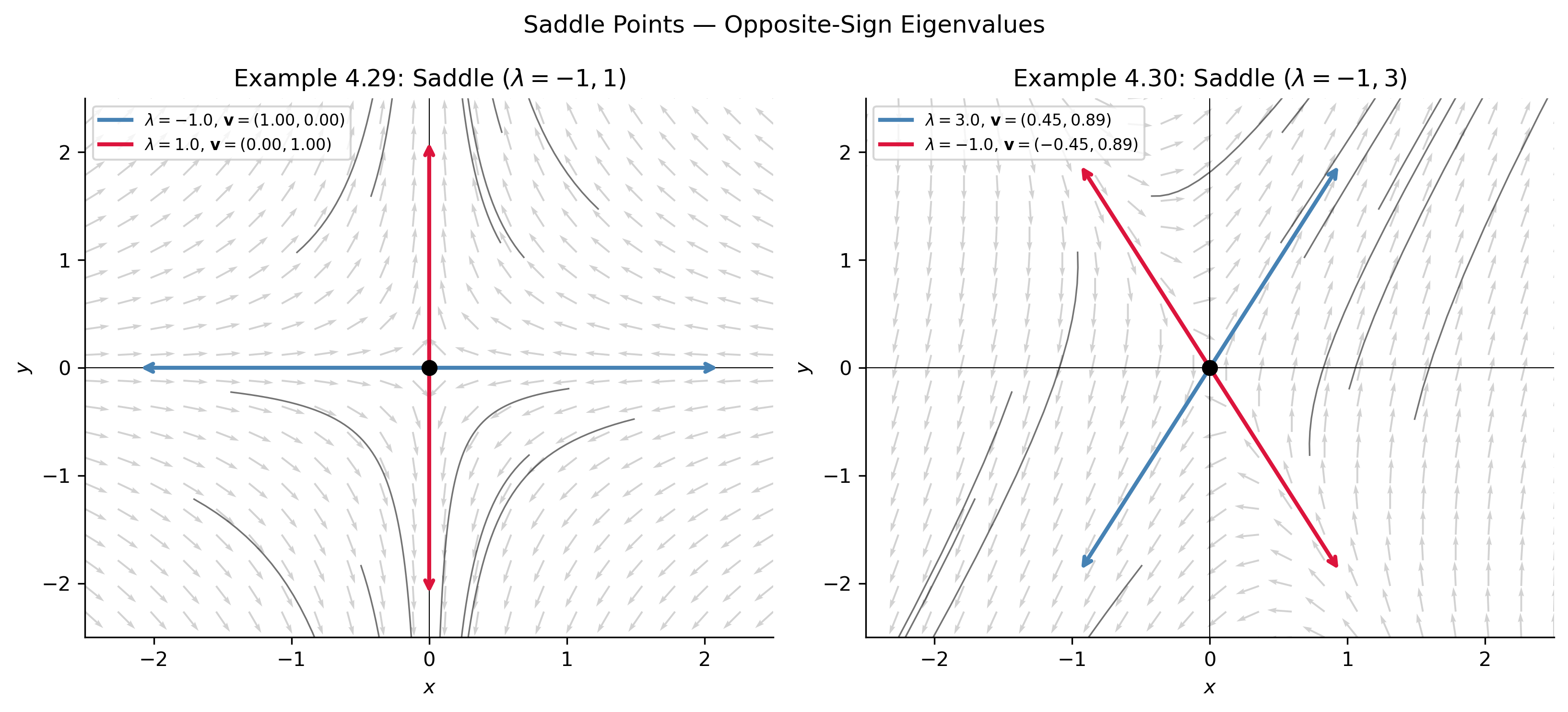
Figure 3: Phase plane portraits for nodal and degenerate cases. Left: asymptotically stable node (Example 4.33, \(\lambda=-1,-6\)) — all orbits enter the origin tangent to the slow eigenvector \(\mathbf{v}_1=(2,1)^T\). Right: \(\det A=0\) case (Example 4.36) — line of equilibria along \(x+2y=0\) with orbits exiting along parallel lines.

Example 4.36 — The Case \(\det A = 0\)

(General solution.) Consider

\[ \mathbf{x}' = \begin{pmatrix}1 & 2\\2 & 4\end{pmatrix}\mathbf{x}. \tag{4.37} \]

The coefficient matrix has \(\det A = 0\), so the characteristic equation is \(\lambda^2 - 5\lambda = \lambda(\lambda-5) = 0\), giving \(\lambda_1 = 0\) and \(\lambda_2 = 5\).

For \(\lambda_1 = 0\): solve \(A\mathbf{v} = \mathbf{0}\), giving \(v_1 + 2v_2 = 0\), so \(\mathbf{v}_1 = (-2,1)^T\).

For \(\lambda_2 = 5\): solving \((A - 5I)\mathbf{v} = \mathbf{0}\) gives \(\mathbf{v}_2 = (1,2)^T\).

The fundamental solutions are \(\mathbf{x}_1(t) = (-2,1)^T\) (a constant!) and \(\mathbf{x}_2(t) = (1,2)^T e^{5t}\), and the general solution is

\[ \mathbf{x}(t) = c_1\begin{pmatrix}-2\\1\end{pmatrix} + c_2\begin{pmatrix}1\\2\end{pmatrix}e^{5t}. \]

The line of non-isolated critical points is in the direction of \(\mathbf{v}_1\), i.e., \(x + 2y = 0\).


Section 4.4.2 — Complex Eigenvalues

If the eigenvalues of \(A\) are complex conjugates \(\lambda = a \pm bi\) (with \(b \neq 0\)), the corresponding eigenvectors are also complex conjugates \(\mathbf{v} = \mathbf{w} \pm i\mathbf{z}\). Taking the eigenpair \(a + bi\), \(\mathbf{w} + i\mathbf{z}\) and expanding via Euler’s formula:

\[ (\mathbf{w} + i\mathbf{z})e^{(a+bi)t} = e^{at}(\mathbf{w} + i\mathbf{z})(\cos bt + i\sin bt) = e^{at}(\mathbf{w}\cos bt - \mathbf{z}\sin bt) + i\,e^{at}(\mathbf{w}\sin bt + \mathbf{z}\cos bt). \]

Since the real and imaginary parts of a complex solution are themselves real solutions, we obtain two real independent solutions:

\[ \mathbf{x}_1(t) = e^{at}(\mathbf{w}\cos bt - \mathbf{z}\sin bt), \qquad \mathbf{x}_2(t) = e^{at}(\mathbf{w}\sin bt + \mathbf{z}\cos bt), \]

and the general solution is

\[ \mathbf{x}(t) = c_1 e^{at}(\mathbf{w}\cos bt - \mathbf{z}\sin bt) + c_2 e^{at}(\mathbf{w}\sin bt + \mathbf{z}\cos bt). \tag{4.38} \]

We need only work with one eigenpair; both give the same pair of real solutions. The factor \(e^{at}\) acts as an amplitude, and the trigonometric factors produce rotation:

  • If \(a < 0\): the amplitude decays and orbits spiral into the origin — the origin is an asymptotically stable spiral point.
  • If \(a > 0\): the amplitude grows and orbits spiral away — the origin is an unstable spiral point.
  • If \(a = 0\) (purely imaginary eigenvalues \(\lambda = \pm bi\)): the amplitude factor is absent, solutions are periodic with period \(2\pi/b\), and orbits are closed ellipses or circles — the origin is a stable center.

Example 4.37 — Asymptotically Stable Spiral

(Complex eigenvalues.) Let

\[ \mathbf{x}' = \begin{pmatrix}-2 & -3\\3 & -2\end{pmatrix}\mathbf{x}. \]

From Example 4.28, the eigenvalues are \(\lambda = -2 \pm 3i\) with eigenvector for \(\lambda = -2+3i\) being \((-1,\,i)^T = (-1,0)^T + i(0,1)^T\), so \(\mathbf{w} = (-1,0)^T\) and \(\mathbf{z} = (0,1)^T\). Applying formula (4.38):

\[ \mathbf{x}_1(t) = e^{-2t}\begin{pmatrix}-\cos 3t\\-\sin 3t\end{pmatrix}, \qquad \mathbf{x}_2(t) = e^{-2t}\begin{pmatrix}-\sin 3t\\ -\cos 3t\end{pmatrix}. \]

The general solution is \(\mathbf{x}(t) = c_1\mathbf{x}_1(t) + c_2\mathbf{x}_2(t)\). Since the real part of the eigenvalue is \(a = -2 < 0\), orbits spiral into the origin as \(t \to +\infty\). At the point \((1,1)\) the tangent vector is \((x',y') = (-5,1)\), so the spirals turn counterclockwise. The origin is an asymptotically stable spiral point. \(\square\)

Show the code
fig, axes = plt.subplots(1, 2, figsize=(11, 5))

def phase_complex(ax, A, title, lim=2.5, t_span=(-0.1, 5)):
    x_g, y_g = np.meshgrid(np.linspace(-lim, lim, 22), np.linspace(-lim, lim, 22))
    dx = A[0,0]*x_g + A[0,1]*y_g
    dy = A[1,0]*x_g + A[1,1]*y_g
    nrm = np.sqrt(dx**2 + dy**2 + 1e-10)
    ax.quiver(x_g, y_g, dx/nrm, dy/nrm, alpha=0.25, color='gray', scale=30)
    np.random.seed(5)
    angles = np.linspace(0, 2*np.pi, 8, endpoint=False)
    for r_frac, color in zip([0.3, 0.7, 1.2], ['steelblue', 'seagreen', 'crimson']):
        for theta in angles[:4]:
            x0 = [r_frac*lim*np.cos(theta), r_frac*lim*np.sin(theta)]
            sol = solve_ivp(lambda t, y: A @ y, t_span, x0,
                           dense_output=True, max_step=0.02)
            xy = sol.y; mask = np.all(np.abs(xy) < lim*1.4, axis=0)
            ax.plot(xy[0, mask], xy[1, mask], color=color, lw=1.3, alpha=0.75)
    ax.axhline(0, color='k', lw=0.5); ax.axvline(0, color='k', lw=0.5)
    ax.plot(0, 0, 'ko', markersize=7, zorder=5)
    ax.set_xlim(-lim, lim); ax.set_ylim(-lim, lim)
    ax.set_xlabel('$x$'); ax.set_ylabel('$y$')
    ax.set_title(title)

# Example 4.37: stable spiral
A437 = np.array([[-2., -3.], [3., -2.]])
phase_complex(axes[0], A437, "Example 4.37: Stable Spiral ($\\lambda=-2\\pm 3i$)",
              t_span=(0, 4))

# Center: purely imaginary eigenvalues lambda = +/- 2i
A_center = np.array([[0., -2.], [2., 0.]])
phase_complex(axes[1], A_center, "Stable Center ($\\lambda=\\pm 2i$)",
              t_span=(0, 2*np.pi + 0.1))

plt.suptitle("Complex Eigenvalues — Spirals and Centers", fontsize=12)
plt.tight_layout()
plt.show()
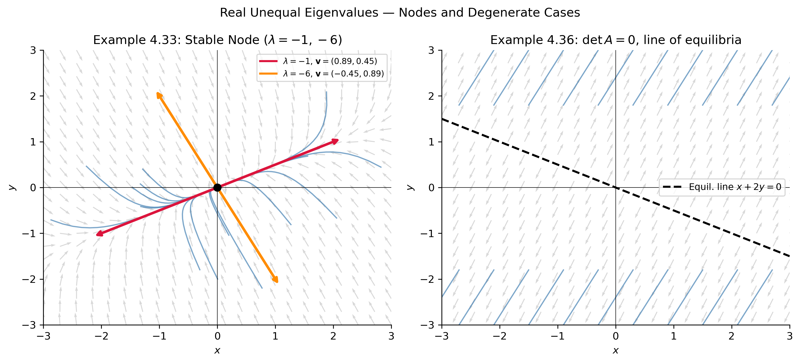
Figure 4: Phase plane portraits for complex eigenvalue cases. Left: Example 4.37 — asymptotically stable spiral with \(\lambda=-2\pm 3i\); orbits spiral into the origin counterclockwise. Right: purely imaginary case \(\lambda=\pm 2i\) — closed elliptical orbits (stable center).

Section 4.4.3 — Real, Equal Eigenvalues

Suppose the eigenvalues of \(A\) are real and equal: \(\lambda_1 = \lambda_2 \equiv \lambda \neq 0\). There are two subcases.

Case 1 (Non-deficient). If \(\lambda\) has two independent eigenvectors \(\mathbf{v}_1\) and \(\mathbf{v}_2\), then there are two independent solutions

\[ \mathbf{x}_1(t) = \mathbf{v}_1 e^{\lambda t}, \qquad \mathbf{x}_2(t) = \mathbf{v}_2 e^{\lambda t}, \]

and the general solution \(\mathbf{x}(t) = c_1\mathbf{v}_1 e^{\lambda t} + c_2\mathbf{v}_2 e^{\lambda t}\) consists of a family of linear orbits along every direction through the origin — a star node (stable if \(\lambda < 0\), unstable if \(\lambda > 0\)).

Case 2 (Deficient). If \(A\) has only a single eigenvector \(\mathbf{v}\) for the repeated eigenvalue, we say the matrix is deficient. Then \(\mathbf{x}_1(t) = \mathbf{v}e^{\lambda t}\) gives one solution. A natural guess of \(t\mathbf{v}e^{\lambda t}\) for the second solution fails. Instead, the second independent solution takes the form

\[ \mathbf{x}_2(t) = e^{\lambda t}(t\mathbf{v} + \mathbf{w}), \]

where \(\mathbf{w}\) is a generalized eigenvector satisfying

\[ (A - \lambda I)\mathbf{w} = \mathbf{v}. \tag{4.39} \]

This system always has solutions because \(\det(A - \lambda I) = 0\). The general solution in the deficient case is

\[ \mathbf{x}(t) = c_1 \mathbf{v}e^{\lambda t} + c_2 e^{\lambda t}(t\mathbf{v} + \mathbf{w}). \]

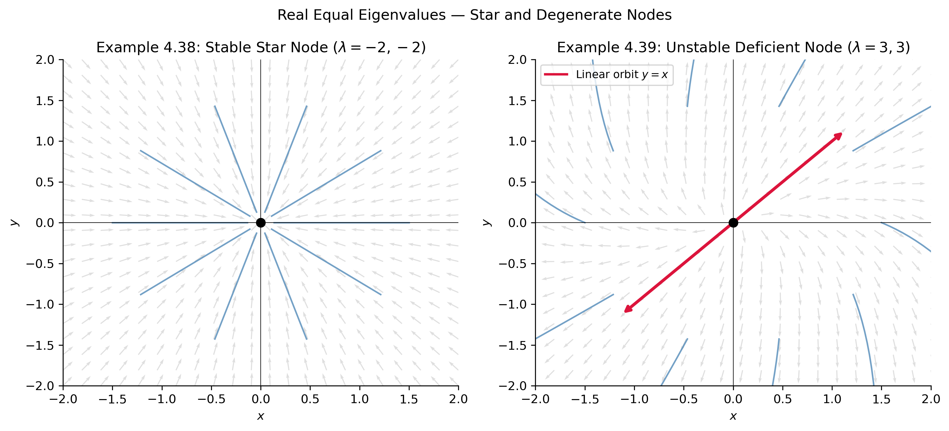
If \(\lambda < 0\), all orbits enter the origin as \(t \to +\infty\) (asymptotically stable node); if \(\lambda > 0\), all orbits exit (unstable node). The term degenerate node is used to describe this structure, as it differs from the common node.


Example 4.38 — Non-Deficient Equal Eigenvalues

Consider

\[ \mathbf{x}' = \begin{pmatrix}-2 & 0\\0 & -2\end{pmatrix}\mathbf{x}. \]

The characteristic polynomial is \((\lambda+2)^2 = 0\) giving \(\lambda = -2,-2\). Substituting \(\lambda = -2\) into \((A - \lambda I)\mathbf{v} = \mathbf{0}\) gives the zero system \(\mathbf{0}\,\mathbf{v} = \mathbf{0}\), so any nonzero vector is an eigenvector. We choose \(\mathbf{v}_1 = (1,0)^T\) and \(\mathbf{v}_2 = (0,1)^T\). The general solution is

\[ \mathbf{x}(t) = c_1\begin{pmatrix}1\\0\end{pmatrix}e^{-2t} + c_2\begin{pmatrix}0\\1\end{pmatrix}e^{-2t}, \]

with components \(x(t) = c_1 e^{-2t}\), \(y(t) = c_2 e^{-2t}\). Their ratio \(y/x = c_2/c_1\) is constant, so all orbits are rays entering the origin (a star node). \(\square\)


Example 4.39 — Deficient Matrix

(Deficient matrix.) Consider

\[ \mathbf{x}' = \begin{pmatrix}2 & 1\\-1 & 4\end{pmatrix}\mathbf{x}. \]

The eigenvalues are \(\lambda = 3, 3\) (repeated). Solving \((A - 3I)\mathbf{v} = \mathbf{0}\):

\[ \begin{pmatrix}-1 & 1\\-1 & 1\end{pmatrix}\mathbf{v} = \mathbf{0} \implies v_1 = v_2, \]

giving the single eigenvector \(\mathbf{v} = (1,1)^T\). One solution is \(\mathbf{x}_1(t) = (1,1)^T e^{3t}\), a linear orbit along \(y = x\).

For the second solution, find \(\mathbf{w}\) satisfying \((A - 3I)\mathbf{w} = \mathbf{v}\):

\[ \begin{pmatrix}-1 & 1\\-1 & 1\end{pmatrix}\mathbf{w} = \begin{pmatrix}1\\1\end{pmatrix}. \]

Both equations give \(-w_1 + w_2 = 1\). Choosing \(w_1 = 0\) gives \(w_2 = 1\), so \(\mathbf{w} = (0,1)^T\). The second solution is

\[ \mathbf{x}_2(t) = e^{3t}\!\left[\begin{pmatrix}1\\1\end{pmatrix}t + \begin{pmatrix}0\\1\end{pmatrix}\right] = \begin{pmatrix}te^{3t}\\(t+1)e^{3t}\end{pmatrix}. \]

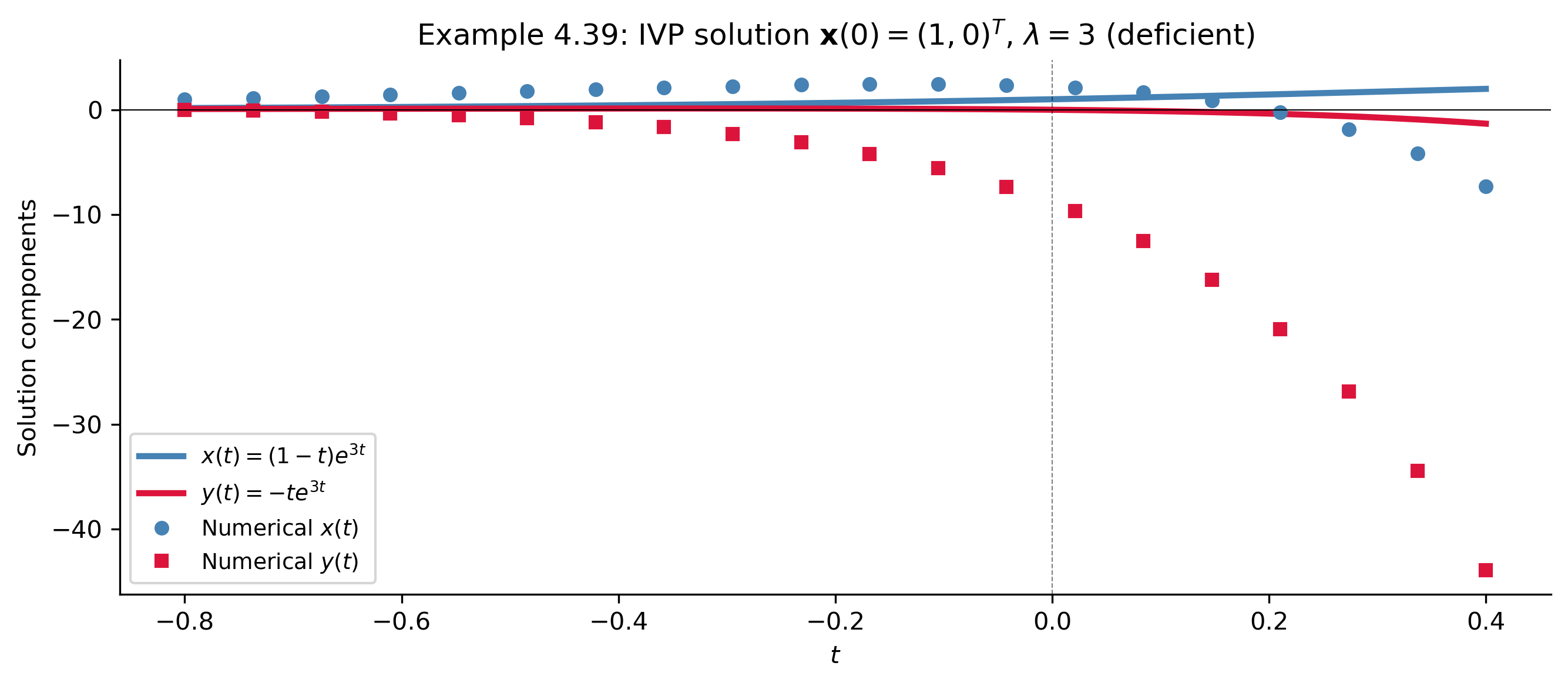
The general solution is \(\mathbf{x}(t) = c_1\mathbf{x}_1(t) + c_2\mathbf{x}_2(t)\). With initial condition \(\mathbf{x}(0) = (1,0)^T\):

\[ c_1\begin{pmatrix}1\\1\end{pmatrix} + c_2\begin{pmatrix}0\\1\end{pmatrix} = \begin{pmatrix}1\\0\end{pmatrix} \implies c_1 = 1,\; c_2 = -1. \]

So

\[ \mathbf{x}(t) = \begin{pmatrix}(1-t)e^{3t}\\-te^{3t}\end{pmatrix}. \]

Since \(\lambda = 3 > 0\), orbits exit the origin — the origin is an unstable node (degenerate). \(\square\)

Show the code
fig, axes = plt.subplots(1, 2, figsize=(11, 5))

# Example 4.38: star node
A438 = np.array([[-2., 0.], [0., -2.]])
lim = 2.0
x_g, y_g = np.meshgrid(np.linspace(-lim, lim, 22), np.linspace(-lim, lim, 22))
for ax, A, title, t_span in [
    (axes[0], A438, "Example 4.38: Stable Star Node ($\\lambda=-2,-2$)", (0, 1.2)),
    (axes[1], np.array([[2., 1.], [-1., 4.]]),
     "Example 4.39: Unstable Deficient Node ($\\lambda=3,3$)", (-0.8, 0))]:

    dx_q = A[0,0]*x_g + A[0,1]*y_g
    dy_q = A[1,0]*x_g + A[1,1]*y_g
    nrm_q = np.sqrt(dx_q**2 + dy_q**2 + 1e-10)
    ax.quiver(x_g, y_g, dx_q/nrm_q, dy_q/nrm_q, alpha=0.25, color='gray', scale=30)

    np.random.seed(99)
    angles = np.linspace(0, 2*np.pi, 10, endpoint=False)
    for theta in angles:
        x0 = [1.5*np.cos(theta), 1.5*np.sin(theta)]
        sol = solve_ivp(lambda t, y, M=A: M @ y, t_span, x0,
                       dense_output=True, max_step=0.02)
        xy = sol.y; mask = np.all(np.abs(xy) < lim*1.4, axis=0)
        ax.plot(xy[0, mask], xy[1, mask], 'steelblue', lw=1.3, alpha=0.75)

    ax.axhline(0, color='k', lw=0.5); ax.axvline(0, color='k', lw=0.5)
    ax.plot(0, 0, 'ko', markersize=7, zorder=5)
    ax.set_xlim(-lim, lim); ax.set_ylim(-lim, lim)
    ax.set_xlabel('$x$'); ax.set_ylabel('$y$')
    ax.set_title(title)

# Highlight the eigenvector direction for deficient case
ax = axes[1]
v = np.array([1., 1.]) / np.sqrt(2)
for s in [1, -1]:
    ax.annotate('', xy=(s*lim*0.8*v[0], s*lim*0.8*v[1]),
                xytext=(0, 0),
                arrowprops=dict(arrowstyle='->', color='crimson', lw=2.5))
ax.plot([], [], 'crimson', lw=2, label='Linear orbit $y=x$')
ax.legend(fontsize=9)

plt.suptitle("Real Equal Eigenvalues — Star and Degenerate Nodes", fontsize=12)
plt.tight_layout()
plt.show()
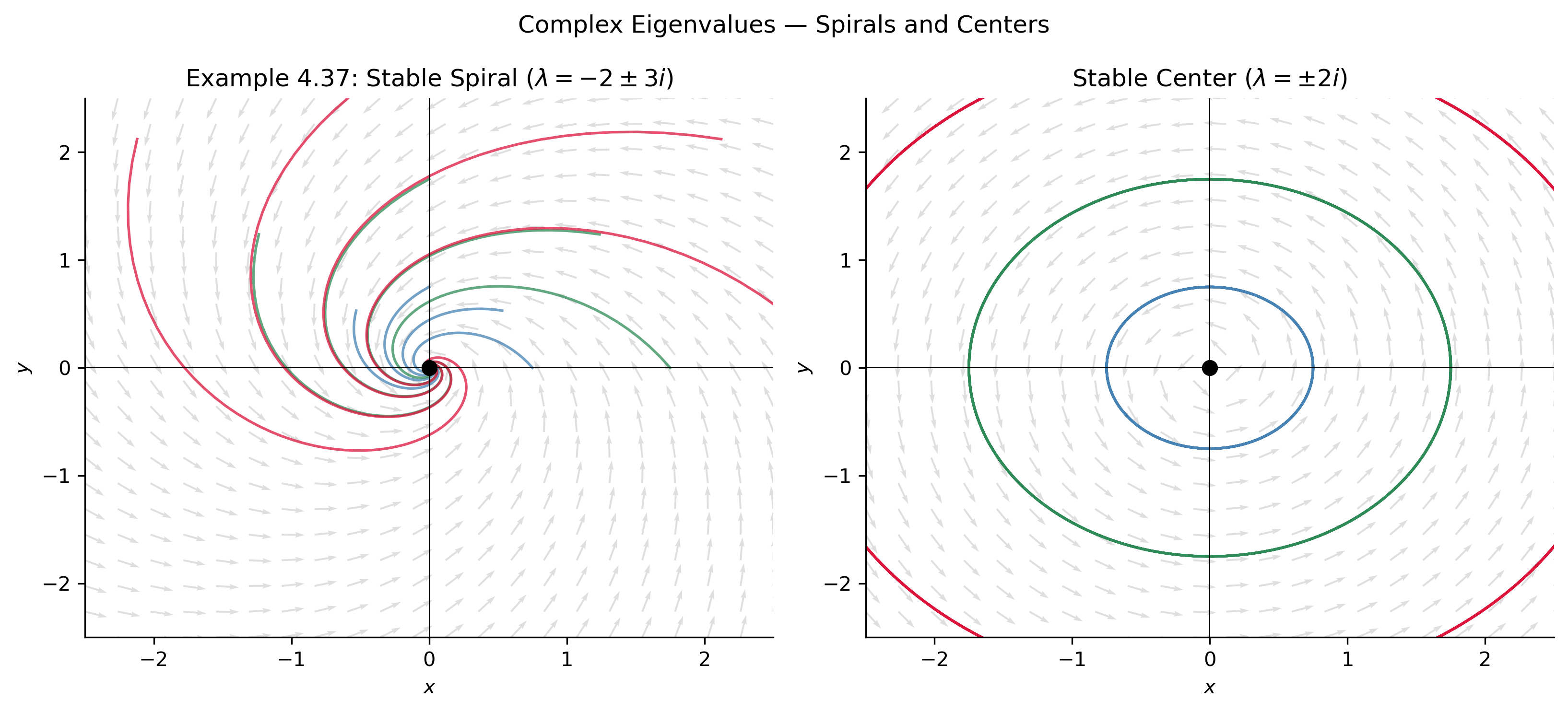
Figure 5: Phase plane portraits for equal eigenvalue cases. Left: Example 4.38 — non-deficient stable star node (\(\lambda=-2,-2\)); every ray through the origin is a linear orbit. Right: Example 4.39 — deficient unstable node (\(\lambda=3,3\)); the single linear orbit is along \(y=x\), and all other orbits curve away.
Show the code
t_plot = np.linspace(-0.8, 0.4, 400)
x_anal = (1 - t_plot) * np.exp(3*t_plot)
y_anal = -t_plot * np.exp(3*t_plot)

A439 = np.array([[2., 1.], [-1., 4.]])
sol = solve_ivp(lambda t, y: A439 @ y, (-0.8, 0.4), [1., 0.],
               dense_output=True, max_step=0.01)
t_dots = np.linspace(-0.8, 0.4, 20)

fig, ax = plt.subplots(figsize=(9, 4))
ax.plot(t_plot, x_anal, color='steelblue', lw=2.5, label=r'$x(t)=(1-t)e^{3t}$')
ax.plot(t_plot, y_anal, color='crimson',   lw=2.5, label=r'$y(t)=-te^{3t}$')
ax.plot(t_dots, sol.sol(t_dots)[0], 'o', color='steelblue', markersize=5, label='Numerical $x(t)$')
ax.plot(t_dots, sol.sol(t_dots)[1], 's', color='crimson',   markersize=5, label='Numerical $y(t)$')
ax.axhline(0, color='k', lw=0.5); ax.axvline(0, color='k', lw=0.5, ls='--', alpha=0.5)
ax.set_xlabel('$t$'); ax.set_ylabel('Solution components')
ax.set_title(r"Example 4.39: IVP solution $\mathbf{x}(0)=(1,0)^T$, $\lambda=3$ (deficient)")
ax.legend(fontsize=9)
plt.tight_layout()
plt.show()
Figure 6: Solution of the IVP from Example 4.39 with \(\mathbf{x}(0)=(1,0)^T\). Both components grow without bound as \(t\to+\infty\), confirming the unstable node. The numerical solve_ivp solution (dashed) exactly matches the analytical formula \(x(t)=(1-t)e^{3t}\), \(y(t)=-te^{3t}\).

Summary

Eigenvalue type General solution form Phase portrait Stability
Real, opposite signs \(\lambda_1 < 0 < \lambda_2\) \(c_1\mathbf{v}_1 e^{\lambda_1 t} + c_2\mathbf{v}_2 e^{\lambda_2 t}\) Saddle — hyperbolic orbits; linear orbits are separatrices Unstable
Both negative \(\lambda_1 < \lambda_2 < 0\) \(c_1\mathbf{v}_1 e^{\lambda_1 t} + c_2\mathbf{v}_2 e^{\lambda_2 t}\) Stable node — orbits enter origin tangent to slow eigenvector Asymp. stable
Both positive \(0 < \lambda_1 < \lambda_2\) \(c_1\mathbf{v}_1 e^{\lambda_1 t} + c_2\mathbf{v}_2 e^{\lambda_2 t}\) Unstable node — orbits exit origin tangent to slow eigenvector Unstable
Complex \(\lambda = a \pm bi\), \(a < 0\) \(c_1 e^{at}(\mathbf{w}\cos bt - \mathbf{z}\sin bt) + c_2 e^{at}(\mathbf{w}\sin bt + \mathbf{z}\cos bt)\) Stable spiral — orbits spiral into origin Asymp. stable
Complex \(\lambda = a \pm bi\), \(a > 0\) Same form as above Unstable spiral — orbits spiral away from origin Unstable
Purely imaginary \(\lambda = \pm bi\) \(c_1(\mathbf{w}\cos bt - \mathbf{z}\sin bt) + c_2(\mathbf{w}\sin bt + \mathbf{z}\cos bt)\) Center — closed ellipses; periodic orbits Stable (not asymp.)
Repeated \(\lambda\), non-deficient \(c_1\mathbf{v}_1 e^{\lambda t} + c_2\mathbf{v}_2 e^{\lambda t}\) Star node — every ray is a linear orbit Asymp. stable (\(\lambda<0\))
Repeated \(\lambda\), deficient \(c_1\mathbf{v}e^{\lambda t} + c_2 e^{\lambda t}(t\mathbf{v}+\mathbf{w})\) Degenerate node — one linear orbit, others curved Asymp. stable (\(\lambda<0\))
\(\det A = 0\), \(\lambda=0\) Constant solution along equil. line Line of equilibria — orbits are parallel lines Not isolated
TipLooking Ahead

The classification of equilibria by eigenvalue type developed here extends directly to nonlinear systems in Chapter 5, where the linearization (Jacobian matrix) at an equilibrium determines local stability. The phase plane for a nonlinear system looks like the linear phase plane near each equilibrium — a fact made precise by the Hartman–Grobman theorem. Centers are the one case where the linearization is inconclusive for the nonlinear system, and the actual behavior must be determined by other means.


These notes are also viewable as a slide deck presentation: Open slides in full screen

Note

Next: Phase Plane Analysis — Logan §4.5.


Relevant Videos

The Eigenvalue Problem:

Solving Linear Systems — Unequal Real Eigenvalues:

Complex Eigenvalues:

Real Equal Eigenvalues:

References

Logan, J David. 2015. A First Course in Differential Equations, Third Edition.
Show the code
import sys
print("Python version:", sys.version)
print('\n'.join(f'{m.__name__}=={m.__version__}' for m in globals().values() if getattr(m, '__version__', None)))
Python version: 3.14.4 | packaged by conda-forge | (main, Apr  8 2026, 02:33:53) [Clang 20.1.8 ]
numpy==2.4.3
sympy==1.14.0
matplotlib==3.10.8

Reuse

CC BY-NC-SA 4.0